by Steven Craighead
 In the prior article, we examined the use of the “cut” function inside of R. This column we examine the “with” command.
The “with” command in R, allows you to quickly evaluate an expression in an environment related to the data. For instance, examining the contents of a data frame, you can use the data frame name and its column name. However, if the data frame name is long, this becomes very tedious. Using the with command, you set up an environment that will permit you to use the data frame once and then just use the variable names separate from the data frame name.
First, we need to simulate a simplified life insurance inforce record set. The R function geninforce is available at Generate Inforce R function. The calling parameters of geninforce are size and randseed. For instance to repeat the results below, use the following command:
inf<-geninforce(1000,10000)
We will also use the R function “subset.” The subset command consists of using a data frame and a conditional term to extract the relative subset. For instance to work with just the female population of the in-force record set, you would use:
subset(inf, gender==”F”)
So, to find the total face of all policies issued to women, use this command:
with(subset(inf,gender=="F"),sum(Face))
[1] 72296587
To find the total reserve of all male smokers, use this:
with(subset(inf,gender=="M" & UWclass=="S"),sum(Reserve))
[1] 89223.67
To demonstrate how the “with” and the “subset” command simplifies the process, this command would have to be used:
sum(inf[inf$gender==”M” & inf$UWclass==”S”,]$Reserve)
[1] 89223.67
The above command doesn’t look too bad, but if the name of the dataframe is longer than three letters, it could become very tedious having to spell it out each time you have to create a subset of the dataframe.
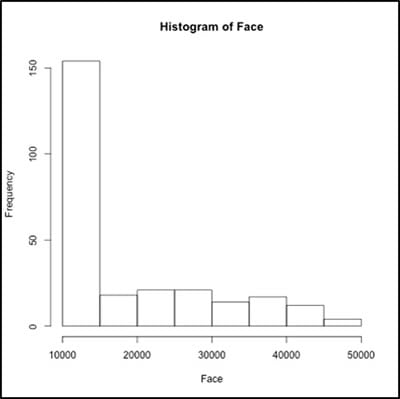
Using the plot command is also helpful. For instance, to obtain the histogram of Face less than 50000, for all females, use this command:
with(subset(inf, gender=="F" & Face<50000), hist(Face))
The graph below should appear:

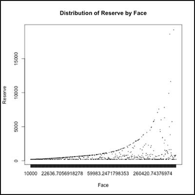
Abusing the boxplot command, we can get an interesting graphic of where the face amount is sorted and the reserves associated with that face are plotted. Using the command
boxplot(inf$Reserve~inf$Face,ylab="Reserve",xlab="Face",
main="Distribution of Reserve by Face")
you will get this graphic:

Using the “with” command, you can easily obtain the same plot by various subsets. For instance this command extracts only the female abused boxplot:
with(subset(inf,gender=="F"),boxplot(Reserve~Face,ylab="Reserve",
xlab="Face",main="Distribution of Reserve by Face"))

You can place a series of commands within a “list” and they will act as if acting on a single command. For instance to obtain the total face, the average premium and the median reserve, you can use this command:
with(inf,list(Face=sum(Face),AvePrem=mean(Premium),MedReserve
=median(Reserve)))
$Face
[1] 172339602
$AvePrem
[1] 1329.706
$MedReserve
[1] 200
The “with” command in R has a great deal of flexibility and power. I recommend that you use the “?with” command and look at other examples within R.
Steven Craighead, CERA, ASA, MAAA, is an actuarial consultant at Pacific Life Insurance. He can be reached at steven.craighead@pacificlife.com.