By Mary Pat Campbell
 The following is an exercise in calculating binomial probabilities, using different approaches in Excel. In honor of my upcoming 40th birthday, I am choosing as the situation to model the case of 2,000 40–year-old women and counting how many die in the next year. Getting my qx from the Social Security 2010 calendar year mortality table, I see the probability for an individual woman is .146 percent. Obviously, most of the probability mass will settle at the low end of the distribution, given that the expected number of dead women is 2.92 and the standard deviation is 1.71.
Before we get into the different approaches, why should you care about knowing multiple ways to calculate a distribution when we have a perfectly good symbolic formula that tells us the probability exactly?
![]()
As we shall soon see, having that formula gives us the illusion that we have the “exact” answer. We actually have to calculate the elements within. If you try calculating the binomial coefficients up front, you will notice they get very large, just as those powers of q get very small. In a system using floating point arithmetic, as Excel does, we may run into trouble with either underflow or overflow. Obviously, I picked a situation that would create just such troubles, by picking a somewhat large number of people and a somewhat low probability of death.
I am making no assumptions as to the specific use of the full distribution being made. It may be that one is attempting to calculate Value at Risk or Conditional Tail Expectation values. It may be that one is constructing stress scenarios. Most of the places where the following approximations fail are areas that are not necessarily of concern to actuaries, in general. In the following I will look at how each approximation behaves, and why one might choose that approach compared to others.
According to Microsoft: http://support.microsoft.com/kb/78113, the smallest representable number in recent versions of Excel is: 2.2250738585072E-308. Well, they say that, but I cannot get to that number exactly. Excel keeps telling me that is zero. It's tough when you're trying to cram a floating point decimal representation into what is really floating point binary. The smallest representable floating point number in my version of Excel is 2 1022, and the largest is (1 + (1 – 2-52)) * 21023 (better known as 1.79769313486232E+308 in decimal.)
To be sure, those numbers are so small and so large that they are generally out of bounds for practical applications. However, one never knows where ever-increasing complexity in actuarial modeling will take you. Understanding the “guts” of one's main calculation engines is important. Even if you use a non–Excel numerical computing solution, there will be floating point limits that one might need to be aware of.
Here are the techniques being tried:
- Binomial Formula
- Excel Function
- Recursion Relation
- Normal Approximation
- Poisson Approximation
- Poisson using Stirling Approximation for n!
- Exponent using Stirling Approximation for n!
Refer to the accompanying spreadsheet Binomial_approximation_examples.xlsx to see (and play with) the results.
1. Binomial Formula
As noted above, the binomial distribution has a closed formula for its probability masses. Why not calculate that directly?
I split the calculation up into steps, so I could see just where it fails (and you will see that it fails).
For the binomial coefficient, I used the COMBIN(number, number_chosen) function. I calculated the exponentiated q and (1-q) in a separate column.
In looking at the spreadsheet tab, we see where it breaks down:
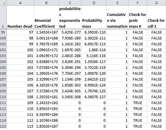
First, we see what is called underflow. In row 111, for 109 dead people, the term (1-q)(N-k) qk falls below the minimum magnitude expressible floating point number for Excel, and therefore is turned into zero ... without any warning.
That's the danger of underflow: in pretty much all floating point systems, it doesn't throw an error. All that happens is a very small, non-zero number resolves as zero.
Here's another problem:
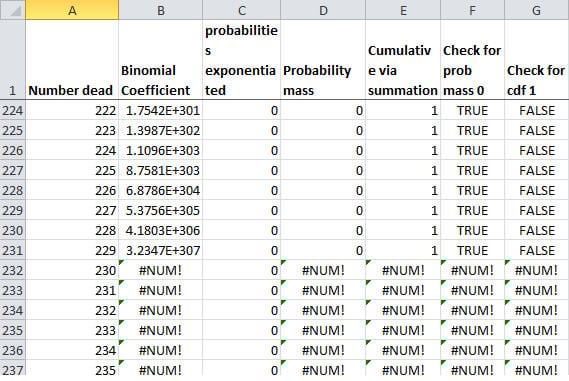
This opposite problem is actually less worrisome: overflow. That's when the number is greater than the maximum magnitude expressible number. That always throws some kind of error in any floating point system, so you can tell when this occurs. However, trying to multiply 0 by #NUM gives you #NUM.
This approach is not necessarily bad, but it does require error-checking so that you get something you can work with. Another problem is that the cdf never reaches 1, and the problem comes well before you hit the underflow issue—the sum tops out at 0.999999999999947. That's pretty close, but still is short about 10 14. That problem comes from trying to add very small magnitude numbers to a much larger magnitude number, during which precision is lost. I will write about that floating point arithmetic issue in a later article.
2. Excel Function
A better solution is to use the built-in Excel function: BINOM.DIST(number_s, trials, probability_s, cumulative). Not only will it give the individual probability masses (set the flag “cumulative” to FALSE—or leave blank, as it is the default option), but also the cumulative distribution (set flag “cumulative” to TRUE). There is no overflow issue with the built–in function.
However, there's still a problem with underflow, and due to the approach taken, the cdf achieves 1 before the probability masses drop to 0.
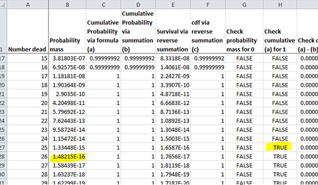
So you can see that BINOM.DIST gives the probability as being above 25 people dying as 0, if you use the cdf option. But it doesn't give non–zero probability if you are calculating probability masses.
For most purposes, BINOM.DIST would be the best choice. Generally one doesn't need precision to the 16th decimal place—it's well beyond the precision we can actually measure. But one must consider how the function actually behaves before you put it into full use.
3. Recursion Relation
Now, we're going to be using more indirect methods from here on out. First, I'm going to try to get around the underflow/overflow problem by noticing that one can put together a recursion relation for the probability mass. I will leave it as an exercise of the reader to derive the following:
When one uses this approach, one gets a result that matches the BINOM.DIST result up to at least 14 decimal places. That's not fabulous, but what's nice is that one doesn't get underflow for the probability mass until 211 people dead, which is the same as BINOM.DIST. Unlike BINOM.DIST, the cdf never reaches one due to the loss of precision when adding small magnitude numbers to much larger ones. Another problem is that if you want to take this approach to calculate a single probability mass (say, 105 people dead), you have to calculate all prior probabilities.
4. Normal Approximation
The next two examples are going to use other probability distributions to approximate the binomial: the normal distribution and Poisson distribution. First, yes, the normal distribution is hideous for this sort of binomial. The problem is that one has too small of a probability of “success” (i.e., death). So the normal distribution is not going to fit the discrete distribution very well.
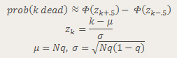
I am using the following approximation for the distribution:
Let's see how well the distribution fits:
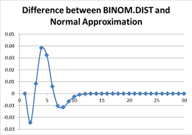
A difference of up to 4 percentage points? And here I was complaining about a difference of the order of 10-14.
There can be some benefits to using a normal approximation in certain circumstances, such as much higher probability of occurrence. When the probability of success is close to 50 percent, and the sample size is large, the normal approximation works much better.
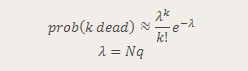
5. Poisson Approximation
The Poisson distribution approximation is generally considered to work best when success probabilities are very close to either 0 or 1 for a binomial. I used the following approximation:
Let's see how well this did:
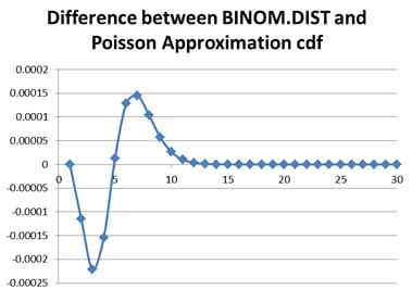
A great improvement over the normal distribution. But there still is a difference of about two bps at the highest–probability items. This level of precision might be warranted given how well our data sets for mortality rates are.
Why would one want to use a Poisson instead of a binomial? Because you may want to be using the number who died as a random variable in a Monte Carlo simulation (involving other dynamics beyond a simple number who died). Say you want to do a one–year projection of cash flows on a block of policies. You can generate a Poisson random variable by assuming constant force of mortality throughout the year—which would have an inter–death time interval simulated by an exponential distribution. One generates exponentials until their sum get you over one year.
6. Poisson with Stirling's Approximation for n!
Now we're going to get weird. In the prior Poisson approximation, I used the built–in POISSON.DIST Excel function. What if we tried using the closed formula for the Poisson distribution directly? Due to the exponentiating, one will get an overflow problem, as well as an underflow problem from a FACT() function call.
What if we used an approximation for factorial within the Poisson approximation itself?
Imagine, if you will, a picture of a smiling Xzibit with the following words imposed over his picture:
" YO DAWG I HEARD YOU LIKE APPROXIMATIONS
SO I PUT AN APPROXIMATION IN YOUR APPROXIMATION "
Whoa, that was weird. It's like the word “approximation” no longer has any meaning.
But back to the story. The Stirling formula approximates the factorial function (or rather the Gamma function, of which factorial is a special case). The resulting combined approximation is below:
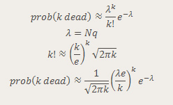
The first two formulas are the regular Poisson distribution, and the third formula is Stirling's approximation to two terms (yes, there are more than two terms there, but I don't want to get into the derivation of this approximation).
The problem, of course, is Stirling's approximation is good only for large values of k. So when I implemented Stirling's approximation, I used it for those items where the overflow/underflow of a directly–calculated Poisson gave me trouble.
There is really no good reason to do what I did here. This was more to demonstrate piecing together different kinds of approximations for different parts of a distribution ... which I will explore more in my next approach.
7. Exponent With Stirling's Approximation For n!
In this next one, I take the piecewise approximation concept even further. I kept an “exact” calculation of the binomial distribution for 14 and fewer people dying, and then used Stirling's approximation for the factorial for higher factorials in the binomial coefficient.
But to provide “extra value,” I used this only as an approximation of the natural log of the probability. You will see this gets around the underflow problem.
Here's my approximation worked out:
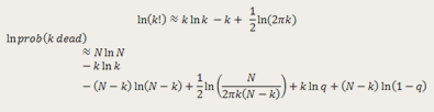
Because I'm working with the natural log of a small number (the probability), and not the small number itself, I don't run into underflow:
So, I am approximating the probability that all 2,000 40–year-old women die in the next year to be about e 13059 … which is probably on the order of the probability of a broken mirror spontaneously repairing itself. Of course, I'm also assuming said 2,000 deaths are independent, but if the Sweet Comet of Death comes screaming from the Oort Cloud, I'm going to guess that independence will be a broken assumption.
Where was I?
So you may be wondering why I am trying to measure probabilities that are so small that we will never have to deal with them in a practical aspect. Part of this is an intellectual exercise for my own amusement, but some of this is trying out some approximation tools in some extreme conditions, to see what “breaks” Excel.
This is to lay groundwork for future articles, looking at how floating point calculation works and techniques to prevent problems like underflow, overflow, and loss of precision. Stay tuned!
Download
Bionomial Approximation Examples Spreadsheet
Mary Pat Campbell, FSA, MAAA, is life analyst for Conning Research & Consulting, Inc. She can be reached at marypat.campbell@gmail.com.