by Steven Craighead
The ability to take continuous data and convert into categories is very useful in actuarial work. This article provides an R function for the calculation of the credibility of mortality claims, and then separates that credibility into different categories using the R cut function.
There are times when working with continuous data that you need to cut the data into groups and use the resultant grouping to model the data. The command in R to do this is the "cut" command. At its simplest, you supply two parameters to this function. The first is a vector of continuous data that you want to group and the second parameter is a vector describing how to make the grouping. The resulting output is a vector of factors reflecting the cuts.
Below, we will use some fabricated mortality data. If you want to replicate the results, you can download the data at:
http://dl.dropbox.com/u/6617438/R Corner Attachments/Raw.csv.
This data reflects only policy count. It has four columns, which are AttainedAge, Sex, Exposed and Deaths. Once you have downloaded the data, you can read it into R by using the read.cvs command:
>Ult<-read.csv("Raw.csv",header=TRUE)
Note: The default cursor in R is ">". All of the commands below, will start with this symbol, but if you are trying to replicate the results in R, just exclude the ">".
A summary of the Ult data.frame is found by using the summary command:
| > summary(Ult) | |||
| AttainedAge | Sex | Exposed | Deaths ; |
| Min. : 55.00 | Female:44 | Min. : 3192 | Min. : 475.8 |
| 1st Qu.: 65.75 | Male:44 | 1st Qu.: 93467 | 1st Qu.: 1240.5 |
| Median :76.50 | Median :138631 | Median : 3499.5 | |
| Mean : 76.50 | Mean : 121439 | Mean : 4542.1 | |
| 3rd Qu.: 87.25 | 3rd Qu.: 167585 | 3rd Qu.: 7481.3 | |
| Max. : 98.00 | Max. : 191230 | Max. : 12272.6 |
Below is a simple function that will calculate the credibility of at different probabilities P and range k:
>Cred<-function(P,k) qnorm((1-P)/2)^2/k^2
For instance, Cred(.9,.05) produces the 1,082 claims that has become the industrial rule of thumb for fully credible claims data. That is if you have 1,082 claims you are 90 percent sure that the total number of claims is within 5 percent (above and below) of the expected claims.
Let's assume that all probabilities will be 90 percent. We will use values of k which will range from 8 percent down to 1 percent. Use this command to create the One vector with eight separate credibility factors:
> One<-round(Cred(.9,8:1/100),0)
> One
[1] 423 552 752 1082 1691 3006 6764 27055
Now add a credibility column to the Ult data frame by using the cut command in this fashion:
>Ult$Credibility<-cut(Ult$Deaths,One)
Summarize this column and you obtain these results:
>options(width=32)
> summary(Ult$Credibility)
(423,552]
3
(552,752]
4
(752,1.08e+03]
11
(1.08e+03,1.69e+03]
11
(1.69e+03,3.01e+03]
11
(3.01e+03,6.76e+03]
20
(6.76e+03,2.71e+04]
28
The "options(width=32)" command shortens the display width, so that the results are displayed vertically. You may restore the width setting to 80 or 132. Note that there are three cells with credibility between 432 and 552, and 28 cells where the mortality is super credible.
Now add a raw mortality column to the Ult data frame with this command:
>Ult$Qx<-Ult$Deaths/Ult$Exposed
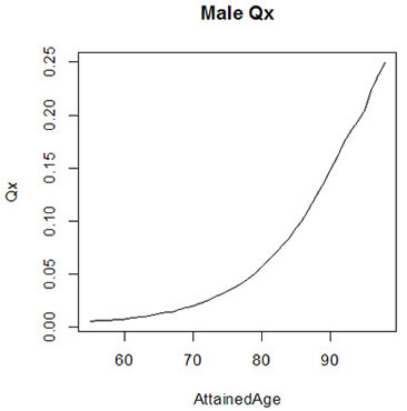
Next plot the raw male mortality rate by attained age by using this command:
> plot(Qx~AttainedAge,data=subset(Ult,Sex=="Male"),type="l",main="Male Qx")
The resulting graphic is:

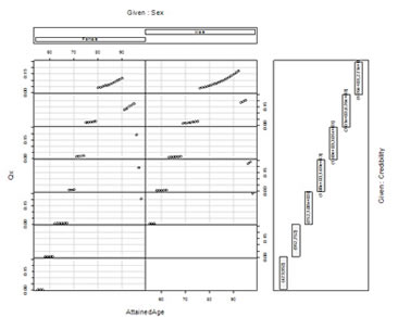
A very interesting graphic is to create a conditional plot for Qx versus AttainedAge conditioned on Sex and Credibility. This is done with this command:
> coplot(Qx~AttainedAge|Sex*Credibility,data=Ult)
The resultant graphic is:

The female mortality by credibility is the graphics on the left hand side of the graph, where the male mortality is in the center of the graphic. Notice on the right hand side how the various credibility levels are displayed. Observe that there is no (423,552] or (552,752] credibility for the male mortality. Also note how much of the raw mortality rates are between ages 80 and 90 for females and 76 to 92 for males. This is where the data is super credible with credibility greater than 6764.
Steven Craighead, CERA, ASA, MAAA is an actuarial consultant at Pacific Life Insurance. He can be reached at steven.craighead@pacificlife.com.