Deep Learning in Segregated Fund Valuation: Part 2

This article is the second part of an article that appeared in April 2022 on the Emerging Topics Community webpage. It will discuss the data preparation, hyperparameter tuning and selection, and the training and testing process of the deep learning models. To reach the final conclusions, the article will continue to compare the projected cash flow results from LSTM and LSTM-Attn with those from the traditional method, and evaluate the time series generations of interest rates and equity returns by WGAN and TCN-GAN.
Training and Testing
Data and Evaluation Metric
For examples of applications of neural network models, we first need to generate the training dataset (Xt,yt). In the first exercise, we used a 12-month window time series where t =1,2 …12. Each risk factor in Xt is generated independently using Monte-Carlo simulation. In the second example, an eight-year time series where t = 1,2 …8 is used. Once the input scenarios are created, they can be fed into AXIS to produce the output value, yt. Market data are utilized to calibrate for the CIR and GARCH stochastic models for scenario generation and to train the GAN models, as follows:
- Canadian Dollar Offered Rate (CDOR), used for CIR calibration and the training of TCN-GAN to produce forward interest rates (1994 to 2021), adjusted by centering at zero.
- Historical monthly TSX/S&P Index close prices, used for GARCH calibration (2001 to 2021) and the training of WGAN-GP to produce future index returns (1985 to 2021).
The deep learning algorithms are trained with 40,000 scenarios of economic risk factors, and 10,000 scenarios separately simulated for validation. To speed up the training process, the training dataset scenarios are grouped into mini batches of five.
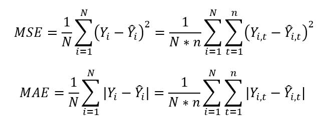
We compare the performance of different cash flow simulation methods (traditional LSMC, LSTM and LSTM-Attn) by two evaluation metrics, mean squared error (MSE), which measures the average squared difference between the estimated and the actual values, and mean absolute error (MAE), which measures the average absolute errors between the estimated and the actual values. For estimates Ŷi ={yi,t}and actual values Yi={yi,t} t=0,...,n i=1,2,...,N samples, they are defined as:
The synthetic returns generated from TCN-GAN and WGAN models are evaluated by distribution and path comparison against the actual historical returns, and the simulated rates from CIR and GARCH models.
Training and Testing
The LSTM model has two major hyperparameters: The number of LSTM layers, and the size of hidden states k; and the FFDNN has three layers with dimensions of l1, l2 and 1 respectively. To speed up the training process, we choose a batch size = 5. After repeating the training process on several combinations, the final hyperparameter settings are selected as: 1 layer of LSTM with k = 300, l1 = 500 and l2 = 100.
In addition to parameters used in the LSTM component, the attention mechanism LSTM-Attn has an additional hyperparameter setting for the dimension of query, key, and value matrices. From our experiments, we chose to use 1 layer of LSTM with k = 400, and for the subsequent FFDNN component of 4 layers with l1 = 500, l2 = 400 and l3 = 100.
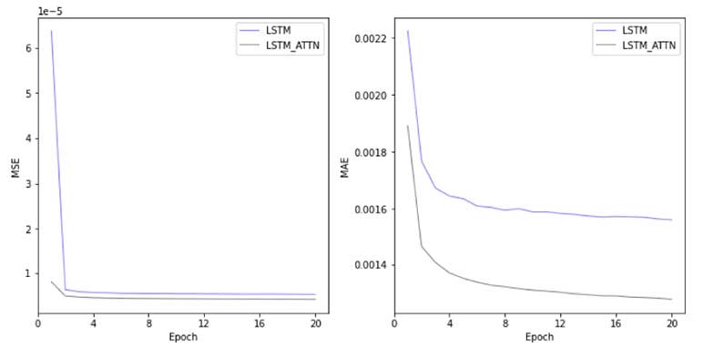
The training process of the LSTM and LSTM-Attn models demonstrates that, subsequent to a sudden drop through the first two epochs, the MSE and MAE performance metrics for both models continuously declined to statistically low levels by 20 epochs, while the LSTM-Attn model consistently outperformed the LSTM model across the epochs. After 20 epochs, the LSTM and LSTM-Attn model results converged sufficiently. (See Figure 5)
Figure 5
Training Process of LSTM & LSTM-Attn by Epoch
Main hyperparameters used in WGAN-GP include the conditional number, which is the number of previous returns used to generate future returns, the time series dimension, which is the total time steps of time series passed into the generator, and the latent dimension controlling the dimension of generated random noises. In our case, we chose a condition number of 5, time series dimension of 17, and latent dimension of 10, and this implies that we use the previous five months return to generate the future 12 months return (in total 17 months), and the returns are transformed by the generator from random noises of dimension 10.
The core hyperparameter used in TCN-GAN specifies the training sample size M, controlling the length of the time series. In our experiment, we chose the sample size of 120 days to train the model. Once the model is trained, the final outputs can be of any dimension, or in other words, the generated time series of interest rates can be of any length.
Results and Comparisons
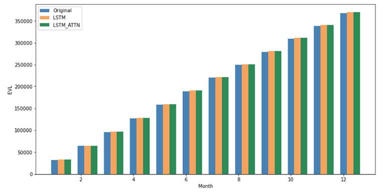
Figure 6 illustrates the result comparison of our deep learning models against the base method (LSMC) and demonstrates that the DL methods have achieved satisfactory degrees of accuracy with errors around 0.1 percent.
Figure 6
Projected Liability Cash Flow Comparison
Additionally, we calculate the one-year economic capital requirements as the difference between VaR(99.95) and the average of projected cash flows (in present value discounted with a discounting rate of 1.79 percent), and find the results of the LSTM and LSTM-Attn models to be lower than the original LSMC results, but still relatively close, with LSTM-Attn producing more precise tail projections, as shown in Table 1.
Table 1
Comparison of Economic Capital Results, One-Year Projection Period
|
|
Original LSMC |
LSTM |
LSTM Attn |
|
Economic Capital @ 1.79% |
106,728.90 |
94,724.21 |
99,161.36 |
The comparison of simulations from WGAN (“fake” returns) against the historical distribution of the in-sample data (“real” returns) in terms of monthly return is illustrated by the histogram of Figure 7.
Figure 7
Comparison of WGAN-GP Simulations and Historical Returns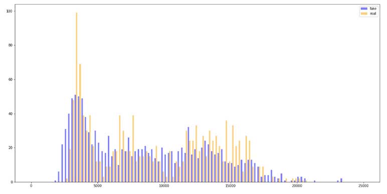
As seen in Figure 8, the back-testing results using overlapped validation data have demonstrated that the simulated distribution by the generator has successfully learned the pattern and correlation between past return and future returns.
We then examine the simulation of future returns by WGAN and compare the simulations with GARCH-BS against the test data in terms of eight-year accumulated return distribution, as shown by the following histograms of Figure 8.
Figure 8
Comparison of Simulated Future Returns, WGAN vs. GARCH-BS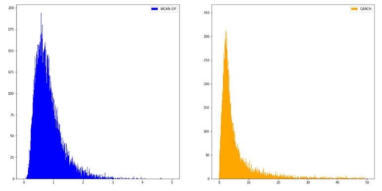
Overall, the distribution of the WGAN simulated returns exhibits similar patterns with the GARCH-BS simulations. However, it is notable that over a relatively long-time horizon, the GARCH model simulates index returns that may accumulate to unreasonably high levels, reaching a maximum 50 times of the initial rate in eight years, further exploding as simulated into longer periods. Meanwhile, the WGAN model can produce accumulated index returns within a reasonable range, supporting it as an improvement to the traditional generators.
The simulation of interest rates generated by TCN_GAN is compared to those by CIR. Interest rates at the end of the eighth year of both methods are shown in Figure 9.
Figure 9
Comparison of Simulated Interest Rate, TCN-GAN vs. CIR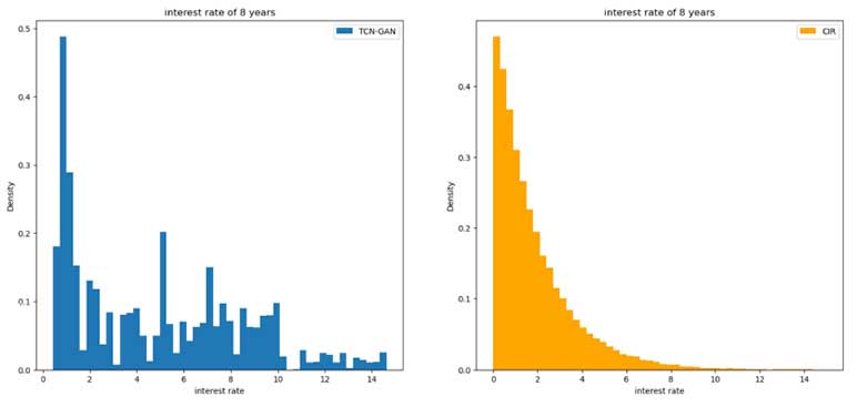
It is found that although both methods generated most values around zeros, the distribution of TCN-GAN contains larger values than CIR. Overall, the distribution of TCN_GAN simulated interest rates exhibits similar patterns with the CIR simulations.
Conclusion
Complicated features of the Seg Fund cash flows have posed computational challenges to the traditional cash flow projection models, such as the nested Monte-Carlo stochastic models, for valuation, capital estimation and pricing purposes. In addition, the current stochastic simulation methods for interest rate and equity return generations, such as CIR and GARCH models, have encountered difficulties for parameter calibrations, and exhibited limitations over long time horizons and for massive scenario generations.
In this article, we demonstrated the applications of deep neural networks techniques based on LSTM and LSTM with Attention models to cash flow projections of Seg Funds, by interpreting the scenarios of interest rate and equity return time series into liability cash flows. Particularly, the LSTM architectures are found to be good solutions to the problem of Seg Fund liability cash flow projection, achieving satisfactory accuracy and enhanced performance efficiency in terms of time and computation requirements. We also experimented with Generative Adversarial Networks for time series generation of interest rates and equity returns, and found that the models succeeded in generating economic scenarios while bypassing the limitations in traditional GARCH and CIR models.
Statements of fact and opinions expressed herein are those of the individual authors and are not necessarily those of the Society of Actuaries, the newsletter editors, or the respective authors’ employers.