Principal Component Analysis Using R

In today’s Big Data world, exploratory data analysis has become a stepping stone to discover underlying data patterns with the help of visualization. Due to the rapid growth in data volume, it has become easy to generate large dimensional datasets with multiple variables. However, the growth has also made the computation and visualization process more tedious in the recent era.

The two ways of simplifying the description of large dimensional datasets are the following:

1. Remove redundant dimensions or variables, and
2. retain the most important dimensions/variables.

Principal component analysis (PCA) is the best, widely used technique to perform these two tasks. The purpose of this article is to provide a complete and simplified explanation of principal component analysis, especially to demonstrate how you can perform this analysis using R.

What is PCA?

In simple words, PCA is a method of extracting important variables (in the form of components) from a large set of variables available in a data set. PCA is a type of unsupervised linear transformation where we take a dataset with too many variables and untangle the original variables into a smaller set of variables, which we called “principal components.” It is especially useful when dealing with three or higher dimensional data. It enables the analysts to explain the variability of that dataset using fewer variables.

Why Perform PCA?

The goals of PCA are to:

1. Gain an overall structure of the large dimension data,
2. determine key numerical variables based on their contribution to maximum variances in the dataset,
3. compress the size of the data set by keeping only the key variables and removing redundant variables, and
4. find out the correlation among key variables and construct new components for further analysis.

Note that, the PCA method is particularly useful when the variables within the data set are highly correlated and redundant.

How do we perform PCA?

Before I start explaining the PCA steps, I will give you a quick rundown of the mathematical formula and description of the principal components.

What are Principal Components?

Principal components are the set of new variables that correspond to a linear combination of the original key variables. The number of principal components is less than or equal to the number of original variables.

In Figure 1, the PC1 axis is the first principal direction along which the samples show the largest variation. The PC2 axis is the second most important direction, and it is orthogonal to the PC1 axis.

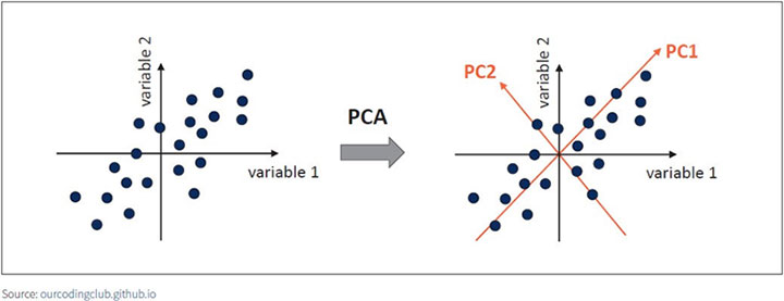
Figure 1 Principal Components

The first principal component of a data set X₁,X₂,...,X_p is the linear combination of the features

Φ_p,1 is the loading vector comprising of all the loadings (ϕ₁…ϕ_p) of the principal components.

The second principal component is the linear combination of X₁,…, X_p that has maximal variance out of all linear combinations that are uncorrelated with Z₁. The second principal component scores z_1,2,z_2,2,z_n,2 take the form

It is necessary to understand the meaning of covariance and eigenvector before we further get into principal components analysis.

Covariance

Covariance is a measure to find out how much the dimensions may vary from the mean with respect to each other. For example, the covariance between two random variables X and Y can be calculated using the following formula (for population):

• xi = a given x value in the data set
• xm = the mean, or average, of the x values
• yi = the y value in the data set that corresponds with xi
• ym = the mean, or average, of the y values
• n = the number of data points

Both covariance and correlation indicate whether variables are positively or inversely related. Correlation also tells you the degree to which the variables tend to move together.

Eigenvectors

Eigenvectors are a special set of vectors that satisfies the linear system equations:

Av = λv

where A is an (n x n)square matrix, v is the eigenvector, and λ is the eigenvalue. Eigenvalues measure the amount of variances retained by the principal components. For instance, eigenvalues tend to be large for the first component and smaller for the subsequent principal components. The number of eigenvalues and eigenvectors of a given dataset is equal to the number of dimensions that dataset has. Depending upon the variances explained by the eigenvalues, we can determine the most important principal components that can be used for further analysis.

General Methods for Principla Compenent Analysis Using R

Singular value decomposition (SVD) is considered to be a general method for PCA. This method examines the correlations between individuals,

The functions prcomp ()[“stats” package] and PCA()[“FactoMineR” package] use the SVD.

PCA () function comes from FactoMineR. So, install this package along with another package called Factoextra which will be used to visualize the results of PCA.

In this article, I will demonstrate a sample of SVD method using PCA() function and visualize the variance results.

Dataset Description

I will explore the principal components of a dataset which is extracted from KEEL-dataset repository.

This dataset was proposed in McDonald, G.C. and Schwing, R.C. (1973) “Instabilities of Regression Estimates Relating Air Pollution to Mortality,” Technometrics, vol.15, 463-482. It contains 16 attributes describing 60 different pollution scenarios. The attributes are the following:

1. PRECReal: Average annual precipitation in inches
2. JANTReal: Average January temperature in degrees F
3. JULTReal: Same for July
4. OVR65Real: of 1960 SMSA population aged 65 or older
5. POPNReal: Average household size
6. EDUCReal: Median school years completed by those over 22
7. HOUSReal: of housing units which are sound and with all facilities
8. DENSReal: Population per sq. mile in urbanized areas, 1960
9. NONWReal: non-white population in urbanized areas, 1960
10. WWDRKReal: employed in white collar occupations
11. POORReal: of families with income less than $3000
12. HCReal: Relative hydrocarbon pollution potential
13. NOXReal: Same for nitric oxides
14. SO@Real: Same for sulphur dioxide
15. HUMIDReal: Annual average % relative humidity at 1pm
16. MORTReal: Total age-adjusted mortality rate per 100,000

The code in Figure 2 loads the dataset to an R data frame and names all 16 variables. In order to define a different range of mortality rate, one extra column named “MORTReal_ TYPE” has been created in the R data frame. This extra column will be useful to create data visualization based on mortality rates.

Compute Principal Components Using PCA ()

PCA () [FactoMineR package] function is very useful to identify the principal components and the contributing variables associated with those PCs. A simplified format is:

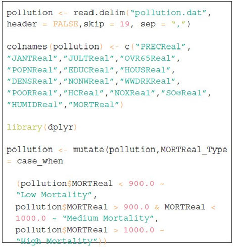
Figure 2 Computer Code for Pollution Scenarios

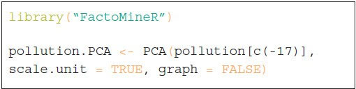
• pollution: a data frame. Rows are individuals and columns are numeric variables
• scale.unit: a logical value. If TRUE, the data are scaled to unit variance before the analysis. This standardization to the same scale avoids some variables to become dominant just because of their large measurement units. It makes the variable comparable.
• graph: a logical value. If TRUE a graph is displayed.

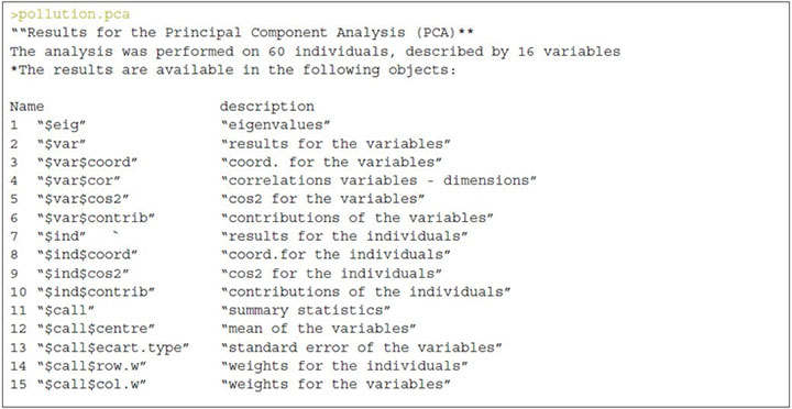
The output of the function PCA () is a list that includes the following components

For better interpretation of PCA, we need to visualize the components using R functions provided in factoextra R package:

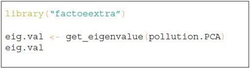
get_eigenvalue(): Extract the eigenvalues/variances of principal components fviz_eig(): Visualize the eigenvalues

fviz_pca_ind(), fviz_pca_var(): Visualize the results individuals and variables, respectively.

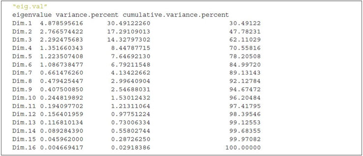
Eigenvalues

As described in the previous section, eigenvalues are used to measure the variances retained by the principal components.

First principal component keeps the largest value of eigenvalues and the subsequent PCs have smaller values. To determine the eigenvalues and proportion of variances held by different PCs of a given data set we need to rely on the R function get_eigenvalue() that can be extracted from the factoextra package.

The sum of all the eigenvalues gives a total variance of 16.

The proportion of all the eigenvalues is demonstrated by the second column “variance.present.”

For example, if you divide 4.878 by 16 equals to 0.304875, i.e., almost 30.49 percent variance explained by the first component/dimension. Based on the output of eig.val object, we can derive the fact that the first six eigenvalues keep almost 82 percent of total variances existed in the dataset.

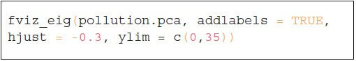
As an alternative approach, we can also examine the pattern of variances using a scree plot which showcases the order of eigenvalues from largest to smallest. In order to produce the scree plot (see Figure 3), we will use the function fviz_eig() available in factoextra() package:

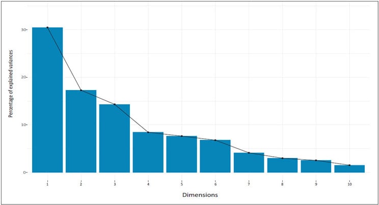
Figure 3 Scree Plot

From the scree plot above, we might consider using the first six components for the analysis because 82 percent of the whole dataset information is retained by these principal components.

Variables Contribution Graph

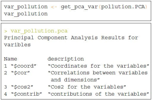
The next step is to determine the contribution and the correlation of the variables that have been considered as principal components of the dataset. In order to extract the relationship of the variables from a PCA object we need to use the function get_pca_var () which provides a list of matrices containing all the results for the active variables (coordinates, correlation between variables, squared cosine and contributions).

Correlation Circle Plot

We can apply different methods to visualize the SVD variances in a correlation plot in order to demonstrate the relationship between variables. The correlation between a variable and a principal component (PC) is used as the coordinates of the variable on the PC.

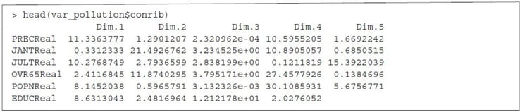
To plot all the variables we can use fviz_pca_var() :

Figure 4 shows the relationship between variables in three different ways:

Figure 4 Relationship Between Variables

• Positively correlated variables are grouped together.
• Negatively correlated variables are located on opposite sides of the plot origin
• The distance between variables and the origin measures the quality of the variables on the factor map. Variables that are away from the origin are well represented on the factor map.

Quality of Representation

This shows the quality of representation of the variables on the factor map called cos2, which is multiplication of squared cosine and squared coordinates. The previously created object var_pollution holds cos2 value:

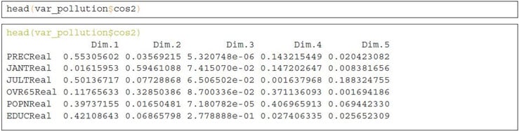
A high cos2 indicates a good representation of the variable on a particular dimension or principal component. Whereas, a low cos2 indicates that the variable is not perfectly represented by PCs.

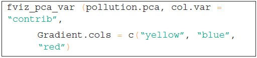
Cos2 values can be well presented using various aesthetic colors in a correlation plot. For instance, we can use three different colors to present the low, mid and high cos2 values of variables that contribute to the principal components.

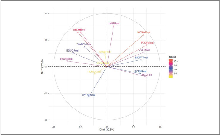
Figure 5 Variables—PCA

Variables that are closed to circumference (like NONWReal, POORReal and HCReal ) manifest the maximum representation of the principal components. However, variables like HUMIDReal, DENSReal and SO@Real show week representation of the principal components.

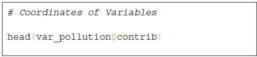
Contribution of Variables to PCS

After observing the quality of representation, the next step is to explore the contribution of variables to the main PCs. Variable contributions in a given principal component are demonstrated in percentage.

Key points to remember:

• Variables with high contribution rate should be retained as those are the most important components that can explain the variability in the dataset.
• Variables with low contribution rate can be excluded from the dataset in order to reduce the complexity of the data analysis.

The function fviz_contrib() [factoextra package] can be used to draw a bar plot of variable contributions. If your data contains many variables, you can decide to show only the top contributing variables. The R code (see code 1 and Figures 6 and 7) below shows the top 10 variables contributing to the principal components:

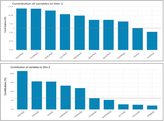
Figures 6 and 7 Top 10 Variables Contributing to Principal Components

The most important (or, contributing) variables can be highlighted on the correlation plot as in code 2 and Figure 8.

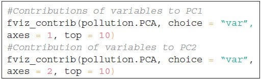
Code 1

Code 2

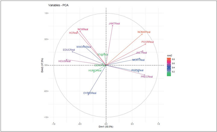
Figure 8 Graphical Display of the Eigen Vector and Their Relative Contribution

Biplot

To make a simple biplot of individuals and variables, type this:

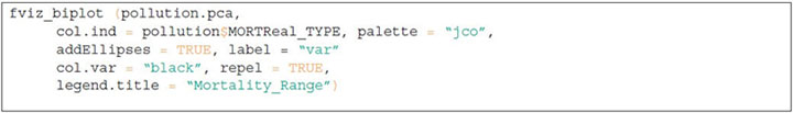
Code 3

In Figure 9, column “MORTReal_TYPE” has been used to group the mortality rate value and corresponding key variables.

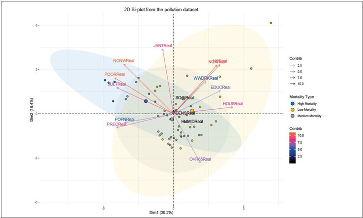
Figure 9 Mortality Rate Value and Corresponding Key Variables Grouped

Summary

PCA analysis is unsupervised, so this analysis is not making predictions about pollution rate, rather simply showing the variability of dataset using fewer variables. Key observations derived from the sample PCA described in this article are:

1. Six dimensions demonstrate almost 82 percent variances of the whole data set.
2. The following variables are the key contributors to the variability of the data set:

   NONWReal, POORReal, HCReal, NOXReal, HOUSReal and MORTReal.

3. Correlation plots and Bi-plot help to identify and interpret correlation among the key variables.

For Python Users

To implement PCA in python, simply import PCA from sklearn library. The code interpretation remains the same as explained for R users above.

Industry Application Use

PCA is a very common mathematical technique for dimension reduction that is applicable in every industry related to STEM (science, technology, engineering and mathematics). Most importantly, this technique has become widely popular in areas of quantitative finance. For instance, fund portfolio managers often use PCA to point out the main mathematical factors that drive the movement of all stocks. Eventually, that helps in forecasting portfolio returns, analyzing the risk of large institutional portfolios and developing asset allocation algorithms for equity portfolios.

PCA has been considered as a multivariate statistical tool which is useful to perform the computer network analysis in order to identify hacking or intrusion activities. Network traffic data is typically high-dimensional making it difficult to analyze and visualize. Dimension reduction technique and Bi- plots are helpful to understand the network activity and provide a summary of possible intrusions statistics. Based on a study conducted by UC Davis, PCA is applied to selected network attacks from the DARPA 1998 intrusion detection datasets namely: Denial-of-Service and Network Probe attacks.

Multidimensional reduction capability was used to build a wide range of PCA applications in the field of medical image processing such as feature extraction, image fusion, image compression, image segmentation, image registration and de-noising of images. Using the multivariate analysis feature of PCS efficient properties it can identify patterns in data of high dimensions and can serve applications for pattern recognition problems. For example, one type for PCA is the Kernel principal component analysis (KPCA) which can be used for analyzing ultrasound medical images of liver cancer ( Hu and Gui, 2008). Compared with the experiments of wavelets, the experiment of KPCA showed that KPCA is more effective than wavelets especially in the application of ultrasound medical images.

Conclusion

This tutorial gets you started with using PCA. Many statistical techniques, including regression, classification, and clustering can be easily adapted to using principal components.

PCA helps to produce better visualization of high dimensional data. The sample analysis only helps to identify the key variables that can be used as predictors for building the regression model for estimating the relation of air pollution to mortality. My article does not outline the model building technique, but the six principal components can be used to construct some kind of model for prediction purposes.

Further Reading

PCA using prcomp() and princomp() (tutorial). http://www.sthda.com/english/wiki/pca-using- prcomp-and-princomp

PCA using ade4 and factoextra (tutorial). http://www.sthda.com/english/wiki/pca-using-ade4-and- factoextra