Deep Learning in Segregated Fund Valuation: Part I

Segregated fund (seg fund) is a type of investment fund administered by Canadian insurance companies. In the form of deferred variable annuity contracts, it offers not only investment capital appreciation like mutual funds, but also predetermined guarantees to the policyholder, including level reimbursement of capital at the maturity of the contract (GMMB) and upon death of the policyholder (GMDB). The pool of investment of seg funds consists of securities such as bonds, stocks, and equity indexes purchased by the insurance company. In nature, seg funds can be referred to as mutual funds with insurance features.

As the value of seg funds fluctuates with the market value of the underlying securities, the insurance company can be adversely affected if the account value drops below the guaranteed levels when their liability increases as the guarantees are in-the-money and payoffs are needed. Economic capital is held to mitigate against market risk, while the projection of capital requirements requires complicated simulation and calculation.

Other business features further add complexity and non-linearity to this process, such as the resetting feature of maturity guarantees that increases the guaranteed level to match higher account values.

Current Methodology in Calculating Capital Requirement

Nested Monte-Carlo-based stochastic models have been used in the calculation of capital requirements, reserving and dynamic hedging for seg fund products by insurers who are allowed to use “internal models” under Solvency II.

The core to these models is the nested stochastic-on-stochastic structure, formed by several “inner” loop scenarios diverging from each of the “outer” loop scenarios at a future time point. The scenarios are simulated by stochastic methods based on underlying economic risk variables from real-world or risk-neutral probability distribution. This two-layer loop of scenarios are then passed into a liability cash flow system (such as AXIS)[1] to project cash flows over the time horizon of the product and then to estimate the desired statistics such as best estimate or Value-at-Risk (VaR). 

Figure 1
Nested Monte-Carlo Model Structure for Seg Fund Cash Flow Projection

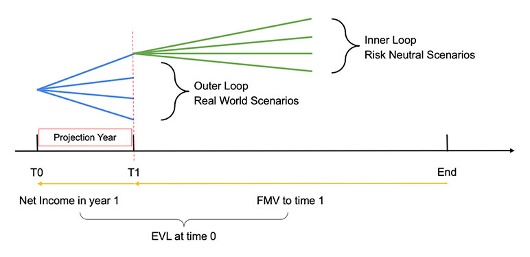
This nested structure has been applied to the valuation of seg funds. The economic value of liability (EVL) of the underlying portfolio is defined as the present value of net cash flows including incomes from fund investment and premiums net of outcomes for expected guarantees and expenses. It is projected as present value at time 0 of the average fair market value of the liability (FMV) across a set of risk neutral “inner” scenarios discounted to the end of year 1 plus the projected net income during the first year from the real world “outer” scenario:

EVL = PV (FMV(t₁)+Y₁ net income)

Further incorporating any hedge credit, the net EVL can then be used for capital requirement calculation, pricing or reserving purposes of seg funds.

For example, economic capital can then be calculated as the difference between the 99.95 percent value-at-risk and the best estimate of projected EVL distribution.

EC = VaR_99.95(EVL) - E(EVL)

The complexity of guaranteed benefit features associated with seg fund calculation-intensive tasks brings considerable computational challenges to the nested loop structure of the full stochastic scenario generation process. Due to the computation constraints of traditional actuarial systems (such as Moody’s GGY AXIS) running the full process on a typical seg fund portfolio can consume a large amount of computational workforce and days of processing time, mostly from the valuation process on inner loop scenarios. AXIS also has the limitation that the same set of scenarios should be used for all seriatim policies in the portfolio, regardless of the specific underlying fund composition or product features.

The Least-Squares Monte Carlo (LSMC)[2] method can be used to significantly reduce the required number of total scenarios through averaging across all inner loop scenarios to achieve an acceptable degree of accuracy as compared with projections from the full approach, and thus improves the efficiency of the valuation process. The valuation of seg funds shows a high similarity to that of the American options. Inspired by the LSMC method, a scenario selection model using linear regression on key variables has been proposed to reduce the processing time of the nested stochastic process.

Deep Learning Methodology

Recent research (1) demonstrated that a deep learning algorithm, Long Short-Term Memory (LSTM), can be trained to project path-dependent cash flows at multiple timesteps of insurance portfolios under various types and combinations of stochastic scenarios. Instead of estimating specific statistics (such as expectation or VaR), the author developed an alternative cash flow model as a multi-purpose solution to various calculation tasks from reserve valuation, risk-based capital calculation and pricing. The nature of the insurance cash flow model shares many similarities with a time series problem as a rule to derive the output time series of cash flows by input time series of multiple risk factors as defined in scenarios. Cash flows predicted at a certain time horizon should also impact subsequent cash flows thereafter. Patterns in the early time range of the scenarios should also continuously affect the predictions for future time. Instead of explicitly expressing all these relationships, the author proved that the LSTM network can simultaneously learn the complexity by selecting information from input scenarios to store in memory for prediction, as demonstrated through two examples of cash flow prediction under different types of scenarios. Test results in the paper showed that the LSTM-based model can achieve a high degree of accuracy in reproducing cash flows with much less computation cost than the traditional Monte-Carlo simulation and LSMC models.

In this article we illustrate in detail how the LSTM algorithm is fitted to capture the non-linear relationship between the output time series of cash flows and the input time series of stochastic economic scenarios. Suitable tuning techniques are applied to tune the projection accuracy in the PyTorch machine learning library. 

We also advance to integrating the attention mechanism to our LSTM network, considering its proven effectiveness in solving the long-time dependency problem of financial time series predictions in recent research (3), and compare the prediction accuracy and model performance of the deep learning models against the original benchmark LSMC model. Finally, we explore the applications of a generative adversarial network (GAN) to the scenario generation of equity returns and interest rates.

In the following sections of this article, we detail our applications of deep learning models to an example block of business composed of seg fund contracts with a mixture of maturity (GMMB) and death (GMDB) guaranteed benefits levels and realistically diversified policyholder characteristics (attained age, gender, anniversary etc.), and compare their results with the benchmark cash flow model applying the LSMC method. We demonstrate that the seg fund cash flows can be predicted using the economic value of net future liabilities as the target output, and the following risk factors as inputs:

• Yield curve of three-month, six-month, 12-month and two-year interest rates: Scenarios generated by the Cox-Ingersoll-Ross (CIR) short rate model.
• Monthly equity index volatility: Scenarios produced by the Generalized Auto Regressive Conditional Heteroskedasticity (GARCH) model.
• Monthly equity index return: Assuming that the stocks follow geometric Brownian motion, a continuous-time stochastic process, calculated as:

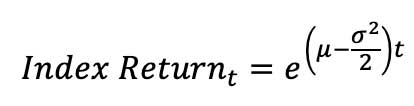
The combination of three risk factors is used as input to our models. The data details refer to the Training and Testing section  that will appear in part II of this article.

LSTM Specialized RNN

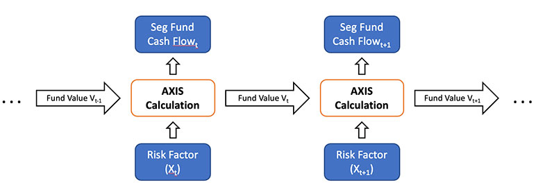
Traditional models for seg fund cash flow calculation are developed in the widely used GGY AXIS platform. At each time step across the policy life, the in-force fund value (V) from the previous step, plus economic risk factors (X) and other static actuarial assumptions from the current step are fed into complicated calculations empowered by AXIS, to project the cash flows, to update policy values after complex policy features such as resetting of guaranteed benefits (G), and to output the fund value from policies in force at the current time point. Mathematically, the relation among risk factors, fund value and our target cash flow can be formulated as follows.

Denote f(•) and g(•) as the embedded computational relationships modeled in AXIS, and V_t, X_t and G_t as the fund value, risk factors and effective guaranteed benefits after any applicable resetting at time t, respectively:

V_t = f (V_t-1,X_t)

Where V₀ is determined based on the initial deposit from policyholder:

Seg Fund Cash Flow_t = g(V_t,G_t)

Figure 2
Cash Flow Projection by GGY AXIS

Such calculation in GGY AXIS is computationally intensive and time consuming, therefore in the industry, some estimation methods proposed to shorten and simplify the process by utilizing estimation models such as multivariate regressions. One limitation of the regression model or any parametric model is that they assume a certain linear or non-linear relationship between risk factors and cash flow outputs. However, complicated product features, such as the guarantee resetting feature, of seg fund policies counter such assumptions as the fund values and cash flows are path dependent. 

In this article, we propose a solution to the path-dependent cash flow projection problem by fitting an LSTM recurrent neural network (RNN), to approximate the unknown function f(•) and g(•).

RNN is widely used in modeling sequential data like language translation and voice recognition. The architecture of RNN makes it also applicable to time series data. LSTM was introduced as a special type of RNN and has shown proven capability of learning long-term dependency through the gating mechanisms in sophistically structured cells. We consider applying the LSTM model to the projection of path dependent seg fund cash flows. 

LSTMs have chain-like structures like RNNs where the previous hidden layer and current input are fed into a cell to produce the next output recursively, with a different design of repeating cells across the time sequence.

Figure 3
Illustration of the LSTM Model Architecture

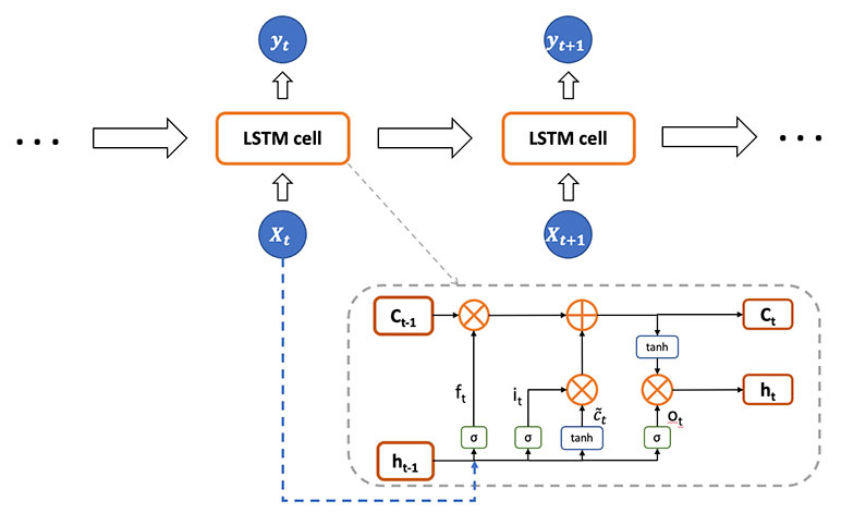
An LSTM cell is composed of an input gate, an output gate and a forget gate, controlling the income and output flow of information in the cell. Mathematically, denote k as the hyperparameter of the dimension of states:

Forget gate: f_t - σ_g(W_fx_t+U_fh_t-1+b_f) ∈ (0,1)^k

Input gate: i_t = σ_g(W_ix_t+U_ih_t-1+b_i) ∈ (0,1)^k

Cell input: i_t = tanh(W_cx_t + U_ch_t-1 + b_c) ∈ (-1,1)^k

Output gate: o_t = σ_g(W_ox_t + U_oh_t-1+b_o) ∈ (0,1)^k

Cell state: c_t = f_t ⋅ c_t-1 + i_t ⋅ c_t ∈ R^k

Hidden state: h_t = o_t · tanh tanh (c_t) ∈ R^k

Where the activation functions are defined as:

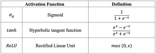
Over the time sequence, the input layer consists of risk factor scenarios, formed as a matrix:

X = [x₁,x₂,...x_n] ∈ R^n×m

where n is the length of time window, m is the number of features. 

The hidden layer stores information from all hidden states across the sequence: 

H = [h₁,h₂,...h_n] ∈ (-1,1)^n×k

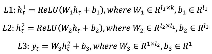
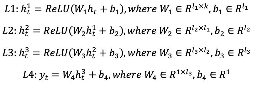
Following the LSTM layers, at time step level, we further incorporated a feed-forward deep neural network (FFDNN) component, consisting of two fully connected layers with ReLU activation functions plus one linear layer to produce the target predictions. 

Prediction: y_t = FFDNN(h_t)

Specifically, FFDNN is composed of a set of layers of neurons. Each neuron of the network is connected to other neurons through a numeric transformation called weight. Additionally, each neuron has an activation function through which it transforms its own global input into output. With predefined dimension hyperparameters and :

The output layer is the predictions from all time steps:

Y= [y₁,y₂,...y_n] ∈ R^n×1

W_* ∈ R^m×k, U_* ∈ R^k×k,b_* ∈ R^k for *∈ {f,i,c,o}, and W_#,b_# f or # ∈ {1,2,3} are parameters that are needed to be learned during the training process.

In our example, x_t consists of three risk factors: Three-month interest rate, equity return and equity volatility at step t, and y_t is the net cash flow over 12 months. The LSTM model learns the relation between x_t and y_t through backpropagation, achieving the same computational functionality with GGY AXIS of cash flow projection. One inherent assumption from the LSTM model is that the learnable parameters are independent of time t across the sequence in a single training scenario. In real business, the underlying relationship between economic risk factors and output cash flows can change from time to time, for example, affected by time-dependent actuarial inputs. However, for an entire portfolio of well-diversified policies, the mathematical relationships can be assumed to remain effectively unchanged across the policy life without expressing explicitly.

LSTM with Attention

A primary constraint of the encoder-decoder based RNN/LSTM networks has been observed that their constitutionally sequential nature limits the model performance in long-range sequence modeling, in that the output at current timestep should represent information from all previous inputs in the sequence as represented by hidden states, resulting in deterioration of the model’s prediction power and performance due to memory constraints at longer time series. 

Attention mechanisms have emerged in deep learning to seek an improvement for long-range sequence modeling. It trains the model to assign different attention weights across the whole input feature sequence and then to selectively align the output with the optimised input sequence. In this way, attention-integrated models have shown proven capability to effectively avoid the long-dependency problem, as well as enhanced model interpretability such as feature importance.

Since its first introduction (4), the attention integrated neural networks have been widely applied to complex sequence learning problems such as image recognition, machine translation and natural language processing. Recent research (3) has also proved the application to financial time series prediction problems of the LSTM network with the integral of attention mechanism. In this article, we consider implementing the LSTM with attention model (LSTM-Attn) to enhance the cash flow model’s performance potential and interpretability.

The architecture of our LSTM-Attn model consists of two components: The attention model and the LSTM model.

Figure 4
Illustration of the LSTM-Attn Model Architecture

 

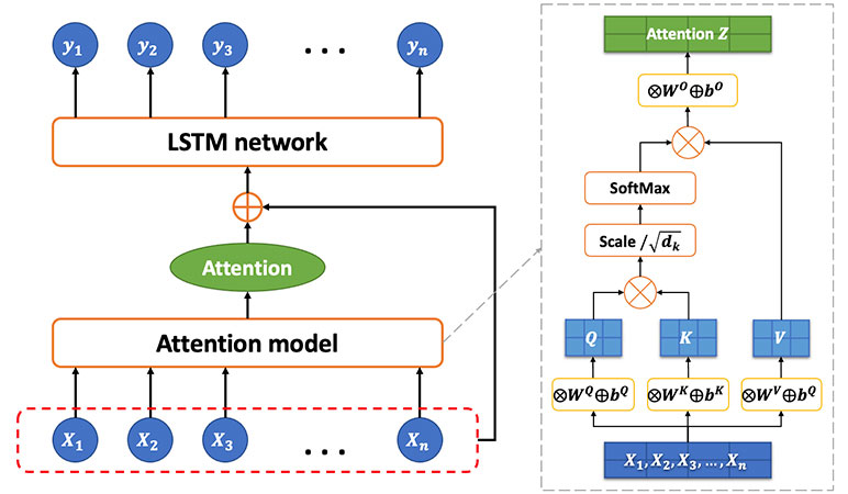
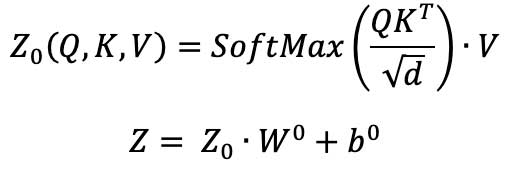
To develop the attention model, we apply the scaled dot-product attention proposed by Vaswani et. al. (2). Specifically, using the query, the key and the value as input, the output attention is calculated as the weighted sum of the values, where the weight assigned to each value is computed by the query and the corresponding key. 

The queries, keys, and values are defined as matrices of dimension md, where m is the number of input features and d is a dimension parameter. The matrices are produced by linear feed forward layers on the input feature sequence, which apply trainable weight matrices W^Q, W^K and W^V and additive trainable biases b^Q , b^K and, b^V:

X ⋅ W^Q + b^Q = Q ∈ R^m×d

X ⋅ W^K + b^K= K ∈ R^m×d

X ⋅ W^V+ b^V= V ∈ R^m×d

Then the dot products are computed of all the queries and keys, each scaled by the square-root of d, and a SoftMax function is applied to the scaled products to calculate the attention scores. Lastly, the dot product of the scores and the values is computed and processed through another linear feed forward layer of weight W⁰ and bias b⁰ to generate the final attention output Z.

The sum of the attention output and the original input sequence is subsequently fed as the newly optimized input sequence into the standard LSTM network, followed by a FFDNN component of three fully connected feed-forward layers plus one linear layer to predict our target values, i.e., the cash flows.

Generative Adversarial Network

In the previous sections we proposed LSTM and LSTM-Attn to predict the cash flow. Another methodology, GAN, has emerged, with promising applications in generative modeling tasks such as object detection, image translation and generations. Recent research has proposed using unsupervised learning techniques such as Wasserstein GAN (5) and Temporal Convolutional Network on GAN for generating synthetic values that follow the probability density of the observed values. 

On top of the WGAN, improved training of Wasserstein GANs was proposed by Ishaan Gulrajani (6) to address the convergence problem in WGAN. In this article, we experiment with the application of WGAN-GP to the simulation of future stock returns as an alternative to complement traditional scenario generation methods such as GARCH. The process is demonstrated as below:

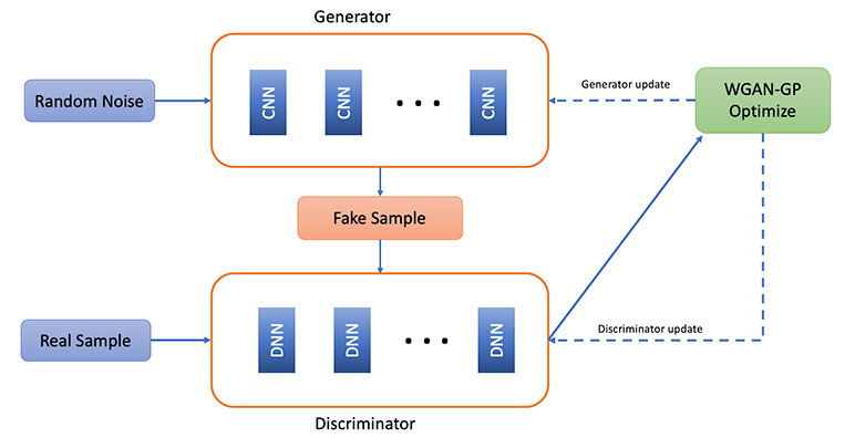
The generator takes random noise and produces synthetic returns based on historical returns. The discriminator takes the return time series from the generator as input and produces the score of the time series. With its generator, it transforms random numbers to real return, and its discriminator is trained to maximize:

L(D,g_θ) = E_x~Pr[logD(x)]+E_x~Pθ[log log (1-D(x))]

By investigating the application of WGAN in the seg fund case, we attempt to find a complementary method to improve the equity return generation by the GARCH model, producing relatively reasonable simulations in terms of return scale over a long-time horizon. Intuitively, the WGAN model works by training the generator to learn to transform randomly generated noises from Gaussian distribution into a synthetic stock return distribution that eventually fools the discriminator, that is, to produce returns that follow the same patterns with the actual historical returns.

We also experiment with the application of Temporal Convolutional Network on GAN (TCN-GAN) as an alternative to the traditional CIR methodology for generating stochastic interest rate scenarios.

TCN is a variation of convolutional neural network, which has recently been shown to be competitive on many sequence modeling tasks. TCNs employ dilated convolutions to capture time series with a long horizon, which insert holes by skipping consecutive elements (7).

In our TCN-GAN model, we employed TCN as the generator. During the training process, the generator is trained using samples of the historical data of the specified size. Random noise that follows a multivariate standard normal distribution is generated. The estimator of the sample, a time series of the length of the training horizon, is then estimated by inferring the random noise through the TCN generator. The discriminator is represented by a TCN with the output being a binary variable of [0,1] to distinguish the estimated time series from the drawn sample data. We train the generator and discriminator iteratively. The whole process of training GAN is summarized in the algorithm below.

Denote G the generator, denote D the discriminator, and M the training sample size. The process of TCN-GAN is described as follows.

(1) Set the learning rates of generator and discriminator as p_G and p_D.

(2) Initialize weight W_G and W_D.

(3) Repeat the following training iterations until convergence:

                Get the training sample from historical input data, X_M ={x₁,x₂ …x_M} ∈R^M

                Generate random noises N_M ={n₁,n₂, …n_M}

Generate the estimator of X_M:

Compute the loss L_D and store the gradient Δ_D that minimize the loss function:  

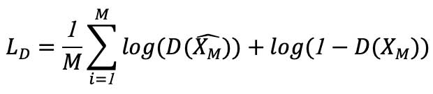Update the discriminator’s parameters: W_D = W_D + p_D ⋅ Δ_D

For every k step, do:

                                Compute the loss L_G and store the gradient Δ_G that minimize the loss function:  

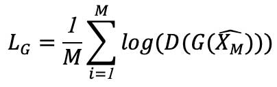
Update the generator’s parameters: W_G = W_G + p_G ⋅ Δ_G

Part 2 of this article will discuss the data preparation, hyperparameter tuning and selection, and the training and testing process of the deep learning models. To reach the final conclusions, the article will continue to compare the projected cash flow results from LSTM and LSTM-Attn with those from the traditional method, and evaluate the time series generations of interest rates and equity returns by WGAN and TCN-GAN.

Statements of fact and opinions expressed herein are those of the individual authors and are not necessarily those of the Society of Actuaries, the newsletter editors, or the respective authors’ employers.