R Corner - Predictive Models and Universal Theorems

By Steve Craighead

There are four universal theorems that I have found to be useful when building models. Two of them are useful when you are doing predictive modeling and the other two are useful when you are modeling statistical distributions.

Universal Theorem One. (Neural Networks) A feed-forward network with a single hidden layer containing a finite set of neurons can approximate continuous functions on compact subsets of Rⁿ. See Wikipedia 1 for more on this theorem.

Universal Theorem Two. (Projection Pursuit Regression). For large values of r and an appropriate set of functions f_j, the PPR model is considered a universal estimator as it can estimate any continuous function in R^p. See Wikipedia 2 for more on this theorem.

These two theorems can give you reassurance in predictive modeling that you can simulate bounded continuous functions using neural networks and any continuous function if you have enough ridge functions f_j.

Universal Theorem Three. (Mixture Distribution). In cases where each of the underlying random variables is continuous, the outcome variable will also be continuous and its probability density function is sometimes referred to as a mixture density. The cumulative distribution function (and the probability density function if it exists) can be expressed as a convex combination (i.e., a weighted sum, with non-negative weights that sum to one) of other distribution functions and density functions. See Wikipedia 3 for more on this theorem.

Universal Theorem Four. (Sklar’s Theorem) Every multivariate cumulative distribution function of a random vector can be expressed in terms of its marginal distributions and a copula. This representation is unique if the marginal functions are all continuous. The inverse of this theorem is also true. See Wikipedia 4 for more on this theorem.

Theorem three indicates that you can model any continuous distribution as a mixture distribution and Sklar’s theorem tells you can model uniquely any continuous multivariate distribution with continuous marginal functions and a copula.

Using universal theorems, you know, even if the models are more complex, that when you build them you can feel more confident in their results.

The rest of the article discusses the use of Theorem One.

Projection Pursuit Regression (PPR)

In linear regression, one fits a response variable Y to a collection of n predictor variables X_i in the familiar form:

In generalized additive models (GAM), the β_iX_i are replaced with various functions f_i(X_i), with this form:

PPR is a modification of this structure in that there are:

1. There are M different f_i.
2. Each f_i acts on a different linear combination of all n of the X_k.
3. A specific coefficient of these linear combinations is denoted by α_ik.
4. Each f_i is multiplied by a β_i.
5. The constant term is the average of the responses.

So PPR takes on the following form:

or in vector format:

Here X = (X₁,X₂,...,X_n) is the predictor vector, and α_i= (α_i1,α_i2,…,α_in).  

The term “projection” in PPR comes from the projection of X on to the directional vector α_i for each i. “pursuit” arises from the algorithm that is used to determine optimal direction vectors α₁,α₂,…,α_M.

Each f_i is called a ridge function. This is because they only have values in the α_i direction and are considered constant elsewhere. Effectively, what occurs is that the overall PPR model is a linear combination (β_i are the coefficients) of the ridge functions. These functions only take on values that arise from the projection of the predictors against the direction vectors, and the functions as assumed to take on a constant value in any other direction. So, each ridge function is like the highest ridge of a mountain range, and we linearly combine these functions along all different ridges (as pointed out by the α_i). Projection pursuit and ridge functions are both subtopics used within the data science field.

On a formal basis, Y and X are assumed to satisfy the following conditional expectation: 

with μ_y = E[Y ] and the f_ihave been standardized to have zero mean and a unit variance. That is: E[f_i(a_i ⋅ X)] = 0 and E[f_i²(a_i⋅ X)] = 1, where i takes on values from 1 to M. We assume that the realized sample values for the random variables Y and X = (X₁, X₂, … , X_n) are independent and identically distributed to the distributions of Y and X, respectively.

The PPR algorithm in the R “stats” library [4] estimates the best β_i,f_i, and the α_i by minimizing the following target function for the mean square error:

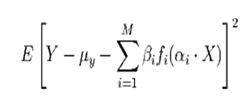
across all the data samples for Y and X.

A powerful trait of PPR models, since the predictor vector X is projected, is that interactions between different X_j and X_kare included within the model, whereas other model algorithms cannot do this without user intervention. This is one of the weaknesses of GAM and GLM predictive models. Let’s look at a justification of this by using an algebraic demonstration based on the S-Plus Guide to Statistics [3] recast into our notation as follows:

Techniques and Diagnostics for PPR

The procedure when using the R PRR algorithm [4] is as follows:

First, one specifies that M should range between M_MIN = 1 and some positive integer M_MAX. The PPR algorithm then creates a PPR model for each M from M_MAXto M_MIN in a descending fashion, and at the same time produces a goodness of fit statistic for each value of M. Scanning this list of goodness of fit values should display a local minimum. If this local minimum is M_MAX one should reprocess the experiment with a larger M_MAX. Once one determines the local minimum, say s, reset M_MIN= s and reprocess the PPR“ppr” algorithm with the same M_MAX as before. The resultant model arising from the backward iteration from M_MAX to M_MINwill then be the best PPR model.

One diagnostic aid in PPR model building is to plot the ridge functions. If these ridge functions are very noisy or discontinuous, you should expect that the resultant PPR model will very likely contain discontinuities.

Another effective diagnostic aid is to both plot the fitted Ŷ against the actual Y and do a simple linear regression of Y against Ŷ, assuming no intercept. The scatterplot should display symmetry around the 45 degree line and the coefficient of the regression should be approximately one. These two diagnostics will indicate how well the PPR model will perform as a predictive model.

Note: A PPR model does not extrapolate outside of the sample data. So, frequently the resultant fitted values from the PPR model will hit a maximum value and will not grow any larger no matter how one manipulates the predictors. This is not the case for linear regression models, where there are no natural limits placed on how one sets any respective X_i. However, one may revise the prediction object to conduct extrapolations. But, one must first feel comfortable with the continuity of the separate ridge functions. If these functions are very noisy or appear not to be differentiable, you might not want to use all extrapolations.

If you want to experiment with PPR, refer to the examples contained in the PPR help section in the “stats” package.

I’ve used PPR extensively in mortality and principle-based reserving, as well as other areas, especially if you want to fit a continuous surface to experience data. Take a look at these articles: Mortality and Principle Based Reserves.

References

[1]  Friedman, J. H. and Stuetzle, W. (1981) Projection pursuit regression. Journal of the American Statistical Association, 76, 817-823.

[2]  Venables, W. N. & Ripley, B. D. (2002) Modern Applied Statistics with S. Springer.

[3]  (2001) S-Plus 6 for Windows Guide to Statistics, Volume 1, Insightful Corporation, Seattle, WA.

[4]  R Development Core Team (2016). R: A language and environment for statistical computing. R Foundation for Statistical Computing, Vienna, Austria. ISBN 3-900051-07-0, URL http://www.R-project.org.