Actuarial Monopoly – bringing Markov home to the family

by Tim Heng

The following is reprinted with permission from Corality Financial Group.

Synopsis

The principle of the long-term steady state is commonly used in actuarial circles, but finds little traction elsewhere. In this article, rather than building financial models for project and investment analysis in my day job as an Associate at Corality Financial Group, I apply a Markov Chain and financial analysis to the humble Monopoly® board and show that there's more to the family game than what meets the eye.

Actuarial Monopoly – bringing Markov home to the family.

I believe that the majority of the readers of this article will be split into two camps: "What does Markov have to do with Monopoly?" and "Yes, I knew all about this already!" If you're part of the latter, then you can jump down to the numbers and compare steady state probabilities and prepare long, angry emails to me about why your models give you different results to mine. If you're part of the former, don't worry – I'll come back and answer that question shortly.

When people think of board games, they usually think of Monopoly. A Google Images search for 'board games' presents me with Monopoly boards (or boxes) in six out of the first ten images presented. It's definitely a staple of most family homes and as anyone who's played the game knows, it frequently results in frustration and tears after five hours of stalemates. This, however, doesn't have to be the case, if you follow the findings in this article and build value accordingly.

Modelling And Monopoly

If you're reading this, I assume you either are an actuary (or actuarial graduate), work with actuaries or you typed 'Monopoly modelling' into Google, and are prepared to do further research if necessary. In any event, you would be familiar with the principles behind a Markov Chain.

For those who can't remember their university definition, a Markov Chain is a system that transits from one state to another within a finite space. In particular, it demonstrates the property that transitions are independent, or memoryless – the probability of moving from one state to another is entirely independent from moves that have occurred previously and based solely on the 'current' state.

Markov Chains are used throughout the actuarial world for dealing with a number of real life problems. The one that I find most interesting is when it is time-homogenous and satisfies the conditions for ergodicity as this allows us to determine a steady state, based on a given transition matrix.If you haven't guessed where we're heading with this, then here it is – a Monopoly board can be translated into a time-homogenous, ergodic Markov Chain, as it demonstrates the necessary properties:

• The board has a finite number of states (squares) with probabilities of transiting between each state
• The game process is irreducible – it is possible to get from any square to any other square
• Each state has a periodicity of 1 (i.e. is aperiodic) – the greatest common denominator of the number of steps to get back to a given square is 1
• The probability of transitions are independent of time (movement around the board is based on rolls and is unchanging)¹

Developing A Transition Matrix

Analysing the probabilities of moving from one state to another allows us to develop a transition matrix associated with a Markov Chain. The probability of transitions from square to square on the board is generally fixed, and a probability of movement relating to specific Chance and Community Chest cards can be estimated by multiplying the probability of landing on said squares by the probability of drawing the specific cards.

A consideration needs to be made in relation to player behaviour. In Monopoly, there is very little player choice in movement as the dice rolls control almost all aspects of transitions. The only influence a player can have is in relation to the length of time spent in Jail. At any point in time while residing in Jail, a player may choose to buy their way out, or roll the dice in an attempt to get out for free. A change in this assumption will have significant impacts on the transition matrix. For example, because rolling 'doubles' will always result in a movement out of Jail, making the assumption that players will not voluntarily pay to leave early will result in a slightly higher probability of transitioning from Jail to even-numbered squares forward.

Is this a reasonable assumption to make? I believe so. In the long-term state of the game, the optimal behaviour is to minimise cash outflow, or alternatively, to maximise the probability of ending a turn in a square without rental costs. In this respect, Jail represents a good value proposition for players, as we will discuss shortly. As such, we can be comfortable in producing a transition matrix using this assumption.

Steady State

The importance of this particular type of Markov Chain lies in its ability to derive a steady state, or the long-term probability that a particular state is active. In Monopoly terms, this is the long-term probability that a square will be landed upon by a player.

We can take our transition matrix and calculate the steady state of our Monopoly Markov process. This provides us with the long-term probabilities of ending turn in each state, based on the assumptions that we've made in setting up our transition matrix. From the list below, we can see that Jail is the most frequently occupied square, followed by a Red property, Go, and then Free Parking, three stations and the three Orange properties in mixed order.

Table header: Steady State probabilities

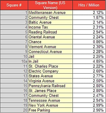
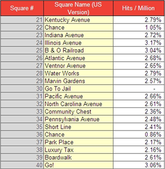
For aficionados of Monopoly, this may seem a bit obvious – 'everybody knows' that the orange and red squares are landed on most commonly, because they are 1-2 rolls from the Jail square, which is visited frequently throughout a game. This general knowledge is backed up by the transition matrix – it is possible to transition from any square to Jail at any point in the game, due to the nature of Chance, Community Chest, the 'Go to Jail' square, and the likelihood of rolling three doubles in a row.

The reasoning behind this is interesting. The red property, square number 24, represented by Trafalgar Square in the UK version or Illinois Avenue in the US version, is the only one of the red properties in the top 10 list. What do we know about this square? It falls exactly 14 steps after Jail, which is the highest probability return from four dice (two turns). There is a Chance card that requires us to move to the square. Understanding the key drivers in the steady state is crucial.

Profit From Applying The Markov Chain

Calculating the steady state is only the first part of the analysis. Knowing where your opponents will land doesn't help you profit from it. We therefore need to consider the income associated with the properties. The expected value can be calculated as the probability of landing in the steady state, multiplied by the rental income from the property. This represents the average income from a property per roll. This is where we see the true value of the Markov Chain analysis.

Table header: Expected value, by square:

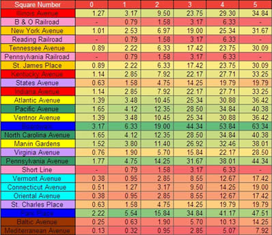
The preceding table shows how we can assess the value of each property based on its income and probability of landing, with green numbers being on the upper range for a given number of houses. Interestingly, despite the higher probability of landing, Illinois Avenue has a very average sort of return. This is because the higher probability is grossly outweighed by the higher rental that you get from more expensive properties – up to double. The best properties, on an expected value basis, are still part of the Dark Blue property group.

So why do we consider Red and Orange to be so good? Because they represent very good value! The next table illustrates how good they are. By looking at payoff tables we can determine how quickly a property will be repaid which in turn show us the return on investment. We calculate the payoff by dividing the cost of purchase / construction by the expected value of the rental income each turn.

Table header: Payoff Period, by Property Group:

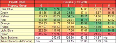
Initially, the Dark Blue property group provides excellent returns on their initial investment. Once the cost of house construction is included, they start to diminish in value, due to the prohibitive cost of building houses on the properties. The same argument applies to the Green property group.

The main reason why people think Red and Orange property groups are the best purchases is because they represent good value in the mid-late stages of the game. The Red property group provides the highest return on investment for properties with 3 houses, and the Orange property group provides the second highest return for properties with 3 or more houses. However, this table shows us something that may be a surprise to you – the Light Blue property group provides very strong investment returns!

Why Steady State Analysis Is Technically Invalid, And Why We'll Use It Anyway!Applying this analysis we now know what is likely to happen if a Monopoly game is played forever. The world record for the longest Monopoly game is 1680 hours – this game definitely reached a steady state!

However, after putting this analysis together, I started running simulations to see if we could translate this into a measure of the probability of winning. In this process, I kept track of how frequently each square was landed on, to compare back to the steady state. This resulted in average landing rates that are relatively different from what we anticipated using the steady state model.

Looking at the average number of turns, we can explain this by showing that the average game doesn't actually run long enough to be able to reasonably use the steady state numbers for a true analysis. The average game only lasts around 40 turns per player before it gets to the end-game scenario, meaning that the probabilities associated with the steady state aren't exactly valid across the whole game when everybody starts off in the same place. To actually obtain my steady state numbers, I had to multiply my transition matrix over 200 times, so a real-world average of 40 turns is woefully small.

So what did we waste all that time for?

Can we still make valid investment decisions based on these calculations? Yes! If we ignore the starting positions, a steady state is a good proxy for having exact probabilities of transitioning to different squares. And if experience says anything, it gives us results that are broadly comparable to anecdotal evidence.

Furthermore, although I needed 200 transitions to get to a steady state, the result was correct to about eight decimal places – a lower level of precision would have been achieved much faster. Although there are technical aspects that invalidate it from being a precisely correct result, it is a sufficiently suitable proxy from a practical point of view.

So now that you're suitably briefed, prepare for your next family gathering and be ready to clean them up!

*MONOPOLY is a registered trademark of Hasbro, Inc.

Tim Heng is an Associate at Corality Financial Group, an analytical consulting firm specialising in advisory, financial modelling, Excel model audits, and training. Tim assists clients with developing innovative solutions to forecasting, operational and financial business problems. He has won an 8 player monopoly tournament at a previous workplace and holds a 55-60% win rate in games played. Tim can be contacted on tim.heng@corality.com, Corality.com. Follow Tim on linkedIn.

¹ Note that this point is slightly false. The transitions are technically dependent on the timing of Chance and Community Chest cards that then get placed at the bottom of the pile, but the impact on analysis is negligible.