Gaining Trust in Predictive Models—an Actuarial Perspective
By David Alison and Wayne Tao
The Financial Reporter, September 2021

With the promise of machine learning and AI also come challenges to successful auditing and evaluation. One challenge is the ability to validate these new models—the more complex the modeling becomes, the more difficult they are for reviewing, communicating, and controlling model risk. Many companies’ model risk management teams struggle to keep up with the pace of change and evolving complexity of models; we are seeing real world examples of where predictive analytics have gone wrong and heightened regulatory expectations are beginning to intersect with the rise of these models.
The explosive growth of computing power over the past several decades has opened an entire new world of possibilities for actuarial predictive models. Innovation in predictive modeling and machine learning has yielded a rich and diverse landscape of modeling tools which actuaries can use to produce more data-driven predictions.
Actuarial model validation must keep pace with the additional complexities from the variety of models that now fall under its scope. While traditional methods like unit testing and static validation continue to be useful, additional methods such as using metadata to track data flows over time or variable significance tests evaluating model structure will become essential for model validation as well.
This article provides an overview of activities that should be considered by an actuary when validating a predictive model. It describes several components to consider when validating a predictive model and provides an examination of various methodologies that can be implemented in the validation process.
Model Selection Methodology
Model selection refers to the selection of the actual modeling technique, components, and functional form to be used in the model. For traditional actuarial models, the model selection stage of the validation process would focus on the choice and reasonableness of assumptions along with how the functionality of the model reflects the problem it is aiming to solve and any limitations in data.
When validating a predictive model, however, the choice of model is often the primary focus. Given the wide variety of possible options when choosing a predictive model or machine learning algorithm, the validator must understand the reason for the selection of a particular model and be able to make an assessment as to whether the model selected was appropriate for its purpose.
When choosing the model, the actuary would be expected to compare alternative solutions and clearly articulate why the given model was selected. In order to understand this model selection process, it’s essential for the validator to understand how various models were ranked, and to make an assessment as to whether the ranking methodologies were correctly applied. (see Figure 1)
Figure 1
The Core Components of Model Selection
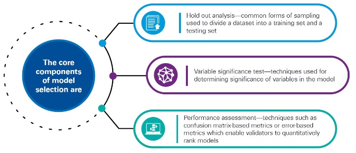
Hold-out Analysis
Hold-out analysis is used to evaluate how the model performs on unseen data, i.e., data that has not been used to calibrate the model parameters. Conceptually, the approach is to remove (or “hold-out”) part of the training/calibration data and compare it to predictions from the model trained/calibrated on remaining data. To assess the accuracy of the prediction, the validator can use performance measures like mean squared error for regression or confusion matrix for classification.
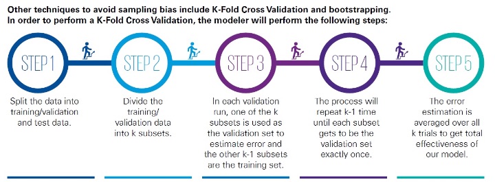
Validators should review the data gathering process and the sampling methodologies to ensure there is no sample bias. Any steps in the data gathering process that could produce a test population that differs from the general population should be understood and considered. Top-sampling—where the top X percent of the sample dataset is selected for training—should be avoided. Instead, random sampling is preferred, where each data point has an equal chance of inclusion in the training set. (see Figure 2)
Figure 2
Steps for K-Fold Cross Validation
Variable Significance Test
Variable significance tests assess the relationship between the predictor variables and the dependent variable. They can be used to reduce the complexity of the model, since insignificant variables may impact the predictive capability in the future, and they can also help validators interpret the model by identifying significant factors. Common techniques include statistical tests, decision trees, and maximal information coefficients.
The p-value is often seen in regression analysis. The p-value for a coefficient tests the null hypothesis that the coefficient is equal to zero (no effect) and it ranges from 0 to 1. A low p-value (< 0.05) indicates that you can reject the null hypothesis. In other words, a predictor that has a low p-value is likely to be a significant addition to the model because changes in the predictor value lead to changes in the dependent variable. (see Figure 3)
Figure 3
Illustrative Example for p-value

In a decision tree model, the variable that the model decides to split on near the root node is significant. In Figure 4 below, family history and body mass index (BMI) are significant in predicting life insurance risk classes.
Figure 4
Illustrative Example for Decision Tree

Maximal information coefficient (MIC), is a measure of the strength of the linear or non-linear association between a predictor variable and response variable. It takes values between 0 and 1, where 0 means statistical independence and 1 means a completely noiseless relationship. The validator can rank the variables by their MICs to identify the significant variables. For example, duration is more significant than moneyness in the MIC table below. (see Figure 5)
Figure 5
Illustrative Example for MIC

Multicollinearity—an Additional Consideration
Multicollinearity could be a problem when the validator assesses the relationship between the predictors and response. Multicollinearity implies highly correlated predictor variables. One common method to detect multicollinearity is to create a correlation matrix with all the variables included in the model. If two variables have a correlation close to ± 1, then often they will be highly correlated. Multicollinearity can also be observed by plotting the variables against each other using a scatter plot—oftentimes relationships can be inferred from patterns in the data.
Performance Assessment
The goal of a successful machine learning model is to use training data to make accurate predictions on data the model has never seen. Both the modeler and the validator must be comfortable that the prediction on training data is accurate while also avoiding overfitting. Overfitting occurs when a model incorporates too much noise or random fluctuations in the training data to the extent that it negatively impacts the performance of the model on new data. This typically happens when the model is too complex due to excessive use of variable transformations and higher power terms.
There are a number of tools that can be used to assess model performance, and so we have included a short list of performance metrics that can be used to assess the goodness of fit and relative performance of the models below:
Akaike information criterion/Bayesian information criterion (AIC/BIC)—functions that measure the fit of the models and penalize the number of parameters included in the model. There is a tradeoff between the complexity and the fit of the model. Complex models with many parameters fit the training data well but are prone to overfitting. A low AIC/BIC score typically strikes a balance, which means a better fit in a less complex model.
Area under the curve (AUC)—this is the area under the receiver operating characteristics (ROC) curve, which is created by plotting the true positive rate against the false positive rate. The higher the AUC, the more accurate the model. A perfect model would have an AUC of 1.
Brier Score—this is the mean squared difference between the predicted probability and the actual outcome. Smaller scores will typically indicate better forecasts.
Confusion matrix—this is typically the foundation for performance metrics for supervised learning models with categorical predictions. Each prediction can be translated into a “positive” or “negative” result, and the confusion matrix compares the positive or negative predictions against the true values that were known from the testing dataset. A model with low false positives and false negatives is better.
Data
One of the primary factors in model selection will be the data. The available computational capacity of cloud computing enables predictive models and machine learning algorithms to consider many more data sources than actuaries have typically worked with in the past. Validators will need to understand relationships between the datasets and assess the relevance of peripheral datasets to the model’s prediction target.
The key components for considering data while validating a predictive model include assessing data lineage, data stability, definitions in the model and the technical requirements of the model, as described below.
Data Lineage
Actuaries need to ensure that data origin (also known as “data lineage”) is well documented. Some methods to accomplish this task include:
- Making use of metadata, which can be gathered at various points in the modeling process;
- ensuring that controls are set up, executed, reviewed, and recorded; and
- relationships between various data sources are well documented and understood.
Data Stability
Various tests can also be conducted to understand how data inputs change over time. This is important because a model may need to be recalibrated or discarded if the model inputs differ too significantly from the original sample that was used to initially calibrate the model.
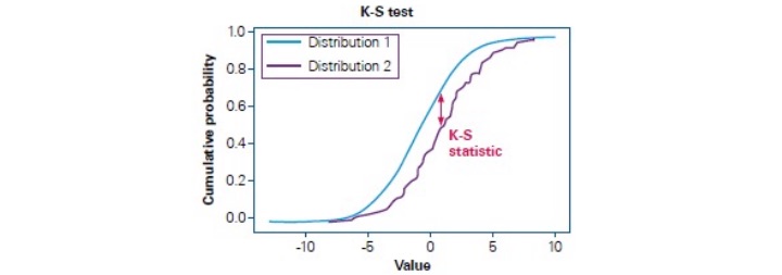
One popular tool to assess changes in data inputs is the Kolmogorov-Smirnov test (K-S test). To conduct this test, the cumulative distribution functions of the inputs to be compared from different samples are plotted on the same graph and the maximum difference is noted. A large maximum difference would indicate that the populations have large distribution differences, whereas a small maximum difference would indicate that the samples are relatively similar. (see Figure 6)
Figure 6
Illustrative Example for K-S Test
Definitions in the Model
Regarding data systems, the actuary will need to review definitions and ensure that they remain consistent throughout the model environment. Changes between model iterations and data pulls also need to be assessed to ensure that data definitions have not been changed, and that any significant changes in field meanings and mappings are thoroughly documented and understood.
Technical Requirements of the Model
In assessing the inputs to the model, the actuary will also need to assess whether the variables follow the technical requirements of the model. The actuary will need to examine the available data and related model outputs by applying expert judgment. One method that the actuary can use to assess whether the inputs relate as expected to the outputs is calculating correlations between the various input variables and the model outputs. If the actuary observes differing correlations between the various input variables and their respective model outputs from various model runs, it is possible that the model is using data inputs inappropriately.
Model Interpretation and Model Tracking
Once the validator is comfortable with the model selection and data inputs of the predictive model or machine learning algorithm, he or she would need to assess model interpretation and model tracking. In some cases, there are limits to the validator’s abilities to interpret the results beyond taking the results as a given. For instance, in a neural network, the many levels of processing can obscure the validator’s expectations of results given the observed inputs. As the results may not be intuitive, the validator would need to leverage tools for assessing error and accuracy in order to make comparisons between the selected model results and results from other models tested.
In the process of considering model tracking, the validator would need to assess and understand how model results change as experience unfolds. The validator would likely need to assess changes in data to determine whether datasets have changed so much that the model is no longer applicable. The K-S test was introduced above as a tool to track changes in distributions over time. This tool can again be used to effectively detect concept drift after a model has been deployed.
The core components of model interpretation and model tracking are interpretability of the model, bias, and model tracking over time, as discussed below.
Model Interpretation
There are several key points the actuary can consider when validating the predictive model’s interpretability.
First, the actuary should be able to understand the outputs, given the inputs. Depending on the model, the parameters chosen for the final model should also give an indication of the model results. For instance, the coefficients of a linear regression indicate the direction and magnitude of the predictors’ impact on the prediction.
Second, the actuary should be able to understand how the model’s predictions would change given changes in the underlying data.
Third, and most obvious, the model should give predictions that make sense. A predictive model that predicts negative mortality clearly is not conceptually sound.
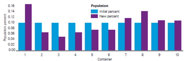
Finally, the actuary should consider evaluating the similarity between the deployed data and training data by looking at summary statistics, making scatter plots to compare variables, and using distribution comparison tools like K-S tests and stability indexes (see Figure 7).
Figure 7
Illustrative Example for Stability Indexes
Model Tracking
Methods for tracking model performance after deployment include rerunning performance tests such as confusion-based metrics to see if performance suffers over time, assessing output distribution changes over time using a stability index, or assessing input distribution changes over time also using a stability index.
The purpose of the stability index is to detect concept drift through changes in the underlying distribution. The stability index measures changes in the model’s predictions by comparing the relative proportions of predictions that fall into prediction buckets. A drastic shift in proportions could indicate that the underlying distributions have changed.
Implementation
Even after the actuary becomes comfortable with model selection, data, and model interpretation and tracking, the actuary still needs to address possibilities of operational risk. This is especially challenging for predictive models due to the heavy use of various programming languages like Python and R, computational requirements, the wide variety of possible models and model evaluation methods, and the possibility that models will be developed by third parties.
Conclusion
Model validation can still be viewed as an emerging field in actuarial science. Model validation of a predictive model adds levels of complexity from the disparate data sources to the need for sophisticated algorithms, to the point that actuarial model validation will need to mature further to account for the additional fluidity and complexity that comes from predictive models.
Model validation for predictive models will require actuaries to develop new skillsets and learn new concepts. Actuaries need to have an understanding of the reason for selecting one model over another, as well as an understanding of how to evaluate the relative performance of the models. Actuaries will need a comprehensive understanding of the end-to-end process of model development, calibration, and assessment in the new age of predictive modeling and machine learning.
David Alison, FIA, is a director at KPMG. He can be reached at davidalison@kpmg.com.
Wayne Tao, is a senior associate at KPMG. He can be reached at guanzhongtao@kpmg.com.