Estimating IBNR for Paid Medical Claims with Zero Run-Out
By Robert G. Lynch
Health Watch, January 2023

The calculation of liability reserves for incurred but not yet paid (IBNR) claims is one of the main functions of the modern health actuary. Due to the great volatility of IBNR estimates calculated by traditional development methods when there is little claims payment run-out, these calculations are typically limited to three months of such run-out. Using the “average paid PMPM” IBNR calculation methodology[1] results in a more robust and consistent estimate of IBNR,[2] but at the expense of ease of use and broadly applicable completion factors. However, in cases where accuracy is desirable over convenience, such as with financial statements, the average paid PMPM method may offer a more consistent estimate than other methods.
The holy grail for IBNR would, of course, be a close measure of IBNR with no claims run-out to make the estimate as timely as possible. While the approach offered here does not truly achieve this high standard, with a mean absolute error of about 5 percent, it gives something of a ballpark estimate of IBNR with no run-out and may serve as the basis for more refined methodology that would come closer to the ultimate objective.
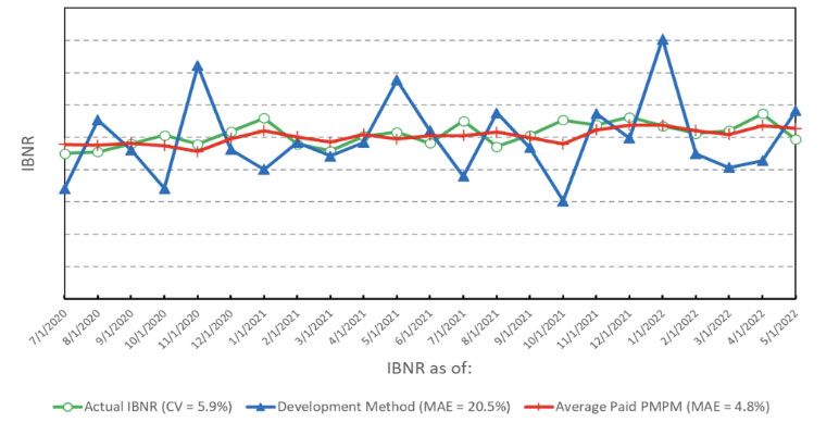
Figure 1 shows the historical performance of the average paid PMPM method compared to a more traditional development approach and the actual IBNR for the commercial medical line of business of a medium-sized, integrated health care delivery organization. The mean absolute error (MAE) for the average paid PMPM method with zero run-out was 4.8 percent over 23 months for a small regional health maintenance organization (HMO), while the development method showed an MAE of 20.5 percent. Results should be better for a larger block of business. The coefficient of variation (CV) of the actual trended paid IBNR values was 5.9 percent.
Figure 1
Zero Run-out Paid IBNR: Actual vs. Development Method vs. Average PMPM Method (Commercial Medical Only)
Methodology
For the calculations in Figure 1, I used 36 months of incurred claims followed through by up to 18 months of paid run-out for each incurred month. Since this results in a rather large 19 by 36 claims lag matrix, I will rely on abbreviated 13 by 24 matrices for illustrating the process in distinct steps. The numbers shown in the steps here are for illustration purposes only and do not reflect any actual claims experience.
A few preliminary data collection and organization steps are needed prior to the main calculation, as described in Step 0.
Step 0: Collect data for adjustment purposes.
- Get counts of covered members by incurral month. These will be used to convert total allowed claims to PMPM amounts in Step 4 and to convert PMPM amounts back to total paid claims in Step 9.
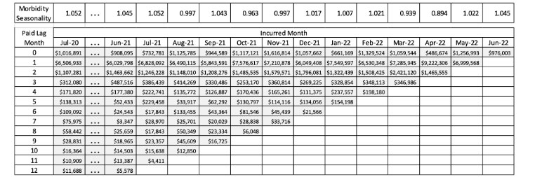
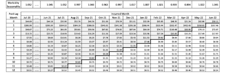
- Average out historical allowed PMPM claims by calendar month, then normalize them to get monthly morbidity seasonality factors that average out to 1. These factors will be used to adjust for seasonality in Step 3. I used four years of data so that each monthly value was based on the average of four separate months of claims.
- Again on a monthly calendar basis, divide average monthly paid claims by monthly incurred claims to get monthly benefit seasonality factors. As with the preceding step, I used four years of data. These factors will be used to convert allowed claims to a paid basis in Step 8.
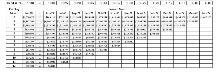
- Estimate a trend rate for adjustment in Step 2. I used an annualized rate of 6.0 percent. It will be used to trend values in Step 2 and also to “de-trend” them in Step 6. Increasing the trend assumption has the effect of increasing the calculated IBNR estimate.
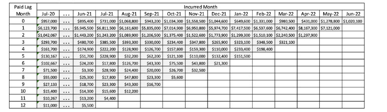
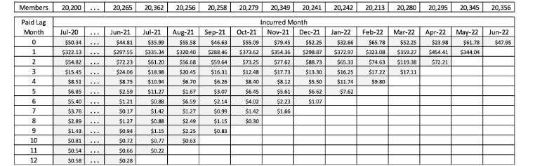
Step 1: Collect total allowed claims by incurred month and paid lag month into the upper-triangular claims lag triangle. I had 36 incurred months and 19 months of paid lag (including lag month 0). So there was 18 months of paid run-out for each incurral month. Table 1 uses 24 incurral months with 12 months of payment run-out, with 10 months of historical data not shown.
Table 1
Step 1: Total Allowed Medical Claims by Incurred Month and Paid Lag Month
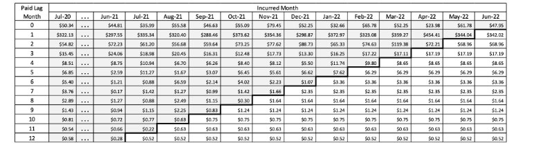
Step 2: Use the estimated trend rate to trend all incurred and paid claims to be on the basis of the final incurred month of the lag triangle. This step serves to put all incurral months on the same temporal basis, as shown in Table 2.
Table 2
Step 2: Total Allowed Medical Claims by Incurred Month and Lag Month Trended to June 2022 at 6 Percent
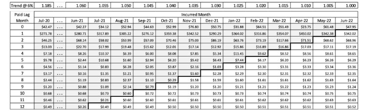
Step 3: Seasonally adjust the allowed claims by applying the calendar month morbidity factors from Step 0(B) to each column, as shown in Table 3.
Table 3
Step 3: Total Seasonally Adjusted Allowed Medical Claims by Incurred Month and Lag Month Trended to June 2022
Step 4: Divide the trended and seasonally adjusted total allowed claims from Step 3 by the number of covered months from Step 0(A) to get PMPM allowed values, as seen in Table 4.
Table 4
Step 4: Seasonally Adjusted PMPM Allowed Medical Claims by Incurred Month and Lag Month Trended to June 2022
Step 5: Fill in the empty lag months in the lower right portion of the triangle by averaging the amounts in each lag row for months that have already been incurred and paid. This step, shown in Table 5, is the core of the average PMPM method.
Table 5
Step 5: Completed and Projected Seasonally Adjusted PMPM Allowed Medical Claims by Incurred Month and Lag Month Trended to June 2022
Step 6: “De-trend” the amounts from Step 5 by applying the trend rate from Step 0(D) in reverse. This step, shown in Table 6, will return the allowed values to their respective nontrended monthly values.
Table 6
Step 6: Completed and Projected De-trended Seasonally Adjusted PMPM Allowed Medical Claims by Incurred Month and Lag Month
Step 7: Remove the seasonal morbidity effects used to average out the PMPM allowed amounts to get back to “actual” allowed PMPM amounts, as seen in Table 7.
Table 7
Step 7: Allowed PMPM Amounts De-adjusted for Seasonal Morbidity Effects
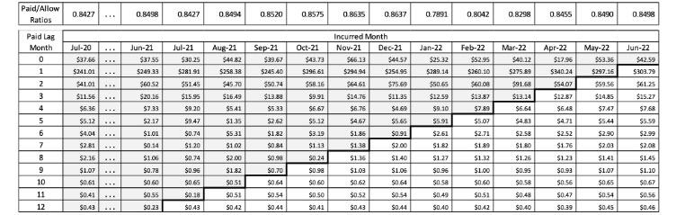
Step 8: Multiply the monthly allowed PMPM claims in every cell of the claims matrix by the benefit factors from Step 0(C) to get estimated PMPM paid claims values, as shown in Table 8.
Table 8
Step 8: Completed and Projected PMPM Paid Medical Claims by Incurred Month and Lag Month
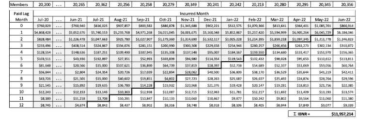
Step 9: Multiply the paid PMPM amounts from Step 7 by the respective monthly member counts from Step 0(A) to get total paid claims by incurral and lag month. Then sum the values in the lower right portion of the claims lag triangle from Step 9, representing the unpaid claims amounts. This value, shown in Table 9, is the IBNR estimate.
Table 9
Step 9: Completed, Trended and Seasonally Adjusted Total Paid Medical Claims by Incurred Month and Lag Month
For the sake of brevity, some of these steps (such as steps 2, 3 and 4, or 6, 7 and 8) may be combined into a single calculation. This will decrease the size of the spreadsheet significantly without affecting accuracy.
Finally, it should be pointed out that, while the approximately 5 percent MAE for this methodology with zero run-out may be a larger error band than is comfortable for all uses, the same methodology can be applied for short run-out periods of one or two months with greater accuracy but with the trade-off of less timeliness. These results may be accomplished by simply leaving the last one or two columns of the matrix from the summed total of IBNR. The methodology shown here may also possibly be combined with nonclaims data (e.g., hospital census data) to improve accuracy.
Statements of fact and opinions expressed herein are those of the individual authors and are not necessarily those of the Society of Actuaries, the editors, or the respective authors’ employers.
Robert G. Lynch, ASA, MAAA, is a data scientist at Dean Health Plan. Robert can be reached at robert.lynch@deancare.com.