Calculation of Confidence Intervals for IBNR Estimates Using the Average PMPM Method
By Robert Lynch
Health Watch, May 2024

In the January 2023 issue of Health Watch, I presented the average PMPM method for calculating incurred but not yet paid (IBNR) values for health claims with no payment run-out. This article is an extension of that methodology to add the calculation of confidence intervals for those IBNR point estimates and is also based in part on Session 4A of the 2023 Society of Actuaries Health Meeting, “Estimating IBNR Reserves with Zero Run-out Using the Average PMPM Method.” The first four steps of the methodology here are identical to the corresponding steps used to determine the point estimate in that article. In brief, those steps are as follows:
- Step 1: Collect total allowed claims by incurred month and paid lag month into the upper-triangular claims lag triangle.
- Step 2: Use the estimated trend rate to trend all allowed claims to be on the temporal basis of the final incurred month of the lag triangle.
- Step 3: Seasonally adjust the allowed claims by applying the calendar month morbidity factor.
- Step 4: Divide the trended and seasonally adjusted total allowed claims from Step 3 by the number of covered member months to get PMPM allowed values.
Step 4 of the example calculation resulted in the allowed claims matrix shown in Table 1.
Table 1
Step 4: Seasonally Adjusted PMPM Allowed Medical Claims by Incurred Month and Lag Month Trended to June 2022 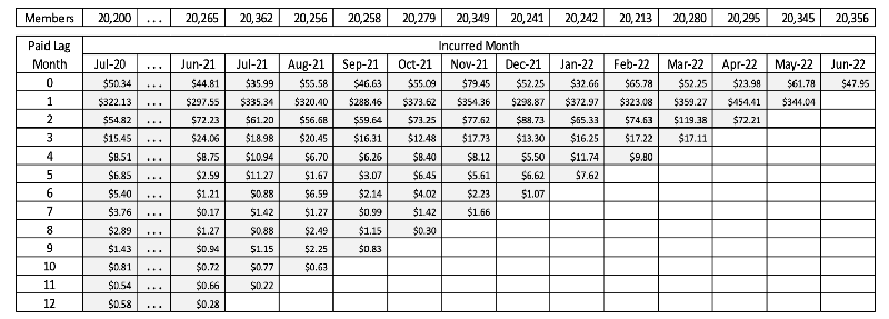
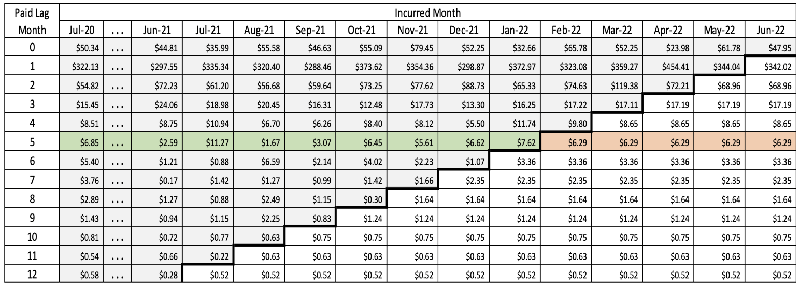
Step 5 of the IBNR point estimate calculation involved projection of the average PMPM IBNR amounts by lag month from the upper left into the lower right portion of the claims completion triangle, resulting in the amounts shown in Table 2 (emphasis added to lag month 5 for clarity of illustration only).
Table 2
Step 5: Completed and Projected Seasonally Adjusted PMPM Allowed Medical Claims by Incurred Month and Lag Month Trended to June 2022
This is the point at which the calculations of the point estimates and the confidence intervals diverge. To get the confidence intervals, this step involves projecting the variances of the lag month lines into the lower left, rather than the average PMPM values, giving the matrix in Table 3.
Table 3
Step 5: Projected Variances of Seasonally Adjusted PMPM Allowed Medical Claims by Incurred Month and Lag Month Trended to June 2022 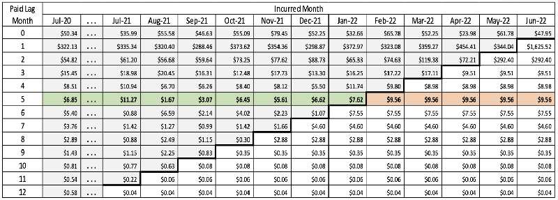
Note: The value of a variance multiplied by a constant is that variance times the constant squared.
The next steps of calculating the confidence intervals are similar to those for calculating the point estimate, with the notable exception that when adjustment constants are applied, the squared value of the adjuster is used rather than simply the direct value. So for detrending the amounts in Step 6, the initial project values from Step 5 are divided by the squared values of the monthly trend factors, as shown in Table 4.
Table 4
Step 6: Detrended Projected Variances of Seasonally Adjusted PMPM Allowed Medical Claims by Incurred Month and Lag Month 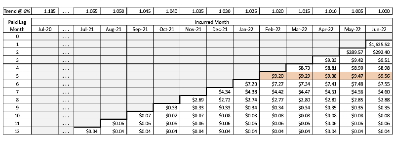
In the next step, the seasonal morbidity effects are removed by multiplying by the square of the seasonal adjustment factors, as in Table 5. For example, the seasonally adjusted value for June 2022 is the variance from Step 6 ($9.56) multiplied by 1.045 squared.
Table 5
Step 7: Variances of Allowed PMPM Amounts Deadjusted for Seasonal Morbidity Effects 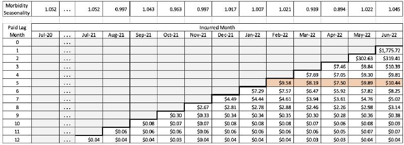
At this point, we start totaling the cell variances to get the total variance of the estimate. However, since the variance of a sum of variances includes adding in twice the covariance, it must first be determined whether the cell values are independent. If they can be shown to be independent, then the covariances are zero. We start by summing the cell variances by incurred month (columns), so to check for independence, it is necessary to regress the PMPM values at lag time t versus the values at lag time t + 1. A coefficient of correlation (R2 value) of less than 0.10 can generally be viewed as indicating independence of the two series. Based on actual experience values, the correlations of the first four lag times are very low, as shown in Figure 1.
Figure 1
Correlations of First Four Lag Times, Paid PMPM values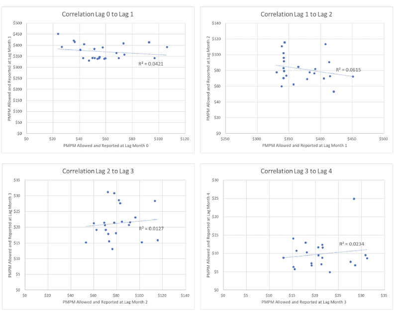
Based on the correlation results shown in this example, the covariances can probably be safely ignored. However, for illustration’s sake, I have included the lag covariances in the calculation. For example, the total PMPM variance for October 2021 (with rounding error) is $0.30 + $0.07 + $0.06 + $0.03 + 2 × (–$0.02 – $0.01 – $0.02) = $0.37. All calculations are shown in Table 6 for Step 8.
Table 6
Step 8: Total Variances of Allowed PMPM Amounts by Incurred Month 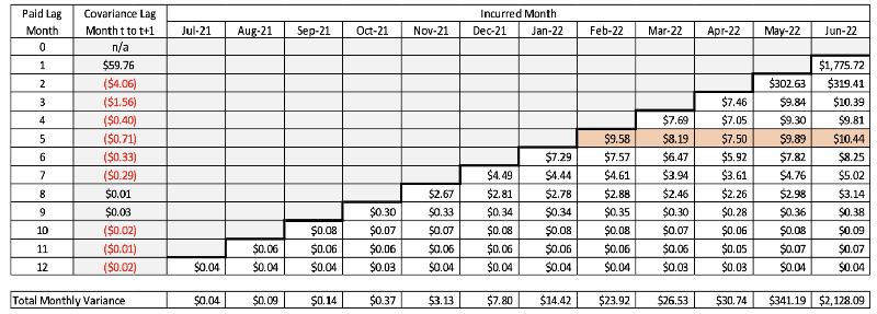
The next step is to convert the monthly variances of allowed claims to paid claims by multiplying the PMPM variances by the squared value of the paid-to-allowed ratio by calendar incurred month, as shown in Table 7. This step also takes care of benefit-based seasonality.
Table 7
Step 9: Projected Total Variances of PMPM Paid Medical Claims by Incurred Month 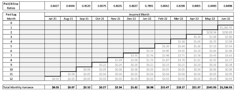
The PMPM variance values then need to be converted to total monthly gross variance by multiplying by the square of the number of member months of exposure in each month, as seen in Table 8.
Table 8
Step 10: Variances of Completed Total Paid Medical Claims by Incurred Month 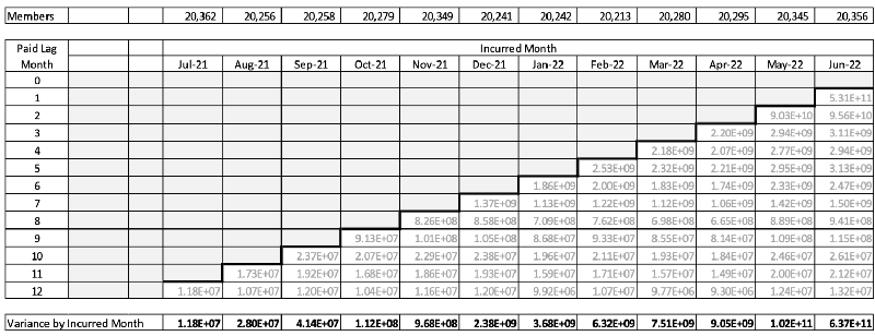
Finally, the total monthly variances are summed together with covariance to obtain the grand total variance for the total IBNR. The covariance is obtained by regressing monthly IBNR values at incurred month t versus values at month t + 1. In this example, there was some correlation for month t to month t + 1, but not for month t to month t + 2 or greater, as shown in Figure 2.
Figure 2
Total Paid PMPM Correlations by Incurred Months 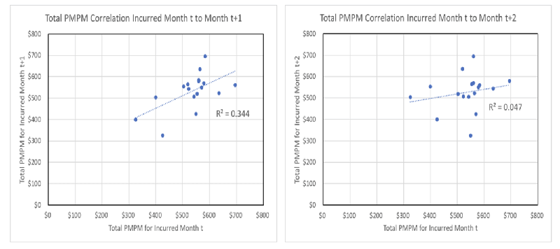
The covariance between incurred month t and month t + 1 in this example is 3,937. Since there are 12 incurred months and 11 effective summations to be made, the grand total variance is the sum of the monthly variances plus 2 × 11 × 3,937, or 7.69 × 10¹¹. The standard deviation is then the square root of the variance, $876,788, and the 95% confidence interval is the point estimate of IBNR ($11,957,214) ± $1,718,505.
To test the reliability of the method, I calculated historical confidence intervals for 36 months of actual data for a regional HMO commercial population of about 175,000 members and found that in 34 of the 36 estimates (94.4%), the actual IBNR fell within the 95% confidence intervals, as shown in Figure 3. In this case, the average 95% confidence interval was ±13.2% of actual IBNR. The mean absolute error of the estimates was 6.4%.
Figure 3
Zero Run-out Paid IBNR—Actual vs. Average PMPM Method with 95% Confidence Intervals (Commercial Medical Only)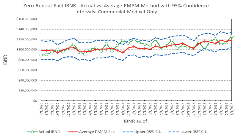
Conclusions
As shown in earlier work, the average PMPM method provides good point estimates of medical IBNR with little or no claims payment run-out time. As shown here, another big advantage of the average PMPM is the ability to easily calculate standard deviations and confidence intervals for those point estimates. With no run-out at all, the 95% confidence interval was on the order of 13.2% for this size block of business, although it would probably be smaller for larger blocks. Based on other research I have done, however, the advantage in accuracy of the average PMPM method over a simple development (completion factor) method decreases as the length of the run-out period increases. The difference is minimal with three months of run-out.
Statements of fact and opinions expressed herein are those of the individual authors and are not necessarily those of the Society of Actuaries, the editors, or the respective authors’ employers.
Robert G. Lynch, ASA, MAAA, can be reached at rgjmcrk@gmail.com.