EWMA Weighted Linear Ridge Regression

By David Romoff

Risks & Rewards, April 2025

Time series forecasting requires balancing adaptability to new data with robustness against overfitting. Traditional methods such as ARIMAX/GARCH or penalized regression address this challenge. This article presents a different quick first-principles approach that integrates Exponentially Weighted Moving Average (EWMA), weighted linear regression, and ridge regression (L2 regularization) into a single closed-form solution.

By applying exponential decay to older observations and shrinking coefficients to manage multicollinearity, this method provides a fast and intuitive tool for short-term forecasting. While it does not capture every structural aspect (autocorrelation or volatility) like ARIMAX/GARCH does, it provides a quick, efficient way to address nonstationarity and overfitting.

Below, each technique is introduced along with matrix-algebra derivations of the resulting regression coefficients. The combined closed-form formula for EWMA-weighted ridge regression is then presented, followed by a discussion of fitting approaches and time-series cross-validation.

Weighted Linear Regression

Weighted regression is a variant of ordinary linear regression in which each observation has a user-specified weight. This approach is beneficial in contexts such as time-series or heteroskedastic data, where some observations may be more important or more reliable than others.

Definitions of the Variables

β: The regression coefficients.
n: The number of observations (rows).
p: The number of predictors (columns) in the design matrix.
The design matrix of predictor variables, where each row x_i^T represents observation i and each column represents a particular predictor.
The response vector, where y_i is the response for observation i.
The weight assigned to observation i, reflecting its relative importance.
A diagonal matrix whose main diagonal entries are the weights. The notation diag(.) refers to the operator that places the given vector elements on the main diagonal of a square matrix, and zeros elsewhere.

Mathematical Intuition and Derivation

Weighted linear regression (WLR) modifies the usual sum of squared residuals by incorporating weights. Specifically, it minimizes

Expanding this expression gives

Taking the gradient with respect to β and setting it to zero leads to

which implies

Larger weights w_i cause the corresponding observations (x_i, y_i) to have a stronger influence on the estimated parameters.

EWMA

EWMA is an approach for weighting observations in a time series so that more recent data carry greater influence than older data. This is especially useful in scenarios where the underlying process evolves over time.

EWMA Formulation and Interpretation

Consider a time series {x_t}. The EWMA is defined by the recursion:

Unrolling this recursion reveals a geometric decay in the influence of past values:

In many financial and statistical contexts, the parameter α is expressed as 1 ‐ λ, with λ denoting the decay factor. Since there is no requirement to normalize these weights for the purposes of linear regression, one can simply express them as a geometric series in terms of λ. The sequence can, therefore, be understood as a geometric series (with common ratio λ) that is not normalized by its sum yet still provides a valid weighting scheme for regression.

Ridge Regression

Ridge regression is a penalized form of linear regression that shrinks coefficients to mitigate collinearity and overfitting. It is especially useful when the design matrix X has closely correlated predictors or when the number of predictors (p) exceeds the number of observations(n) .

Mathematical Intuition and Derivation (L2 Penalty)

Ordinary least squares determine β such that

Ridge regression adds an L2 penalty leading to

Writing

taking derivatives, and setting them to zero gives

The scalar λ scales the strength of the penalty relative to the residual sum of squares. The optimal choice of λ is typically determined via an out-of-sample or cross-validation procedure.

L1 vs. L2, and Standardization

Penalty functions can be of two primary types:

L1 (Lasso): This penalty may drive some coefficients to zero (sparsity) but does not have a closed-form solution.
L2 (Ridge): This penalty shrinks all coefficients continuously toward zero (though not exactly to zero) and does have a closed-form solution.

Standardizing each predictor is generally recommended, so that the penalty applies uniformly across coefficients. This ensures that predictors on vastly different scales are not penalized disproportionately.

EWMA-Weighted Ridge Regression

This section combines weighted linear regression and ridge regression, letting the weights themselves follow an EWMA decay pattern over time. Suppose there are n observations indexed by time, and each observation t has an EWMA-based weight . Collect these into

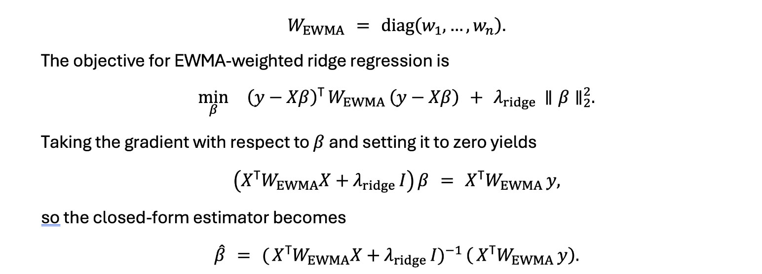
Hence, each data point is downweighted exponentially by age, while the ridge penalty shrinks coefficients to reduce variance and collinearity issues.

Fitting Approach and Cross-Validation in Time Series

Two hyperparameters must be tuned:

(the decay factor for exponential weighting),
(the L2 penalty coefficient).

These are chosen via an out-of-sample approach. In time series, a rolling or forward-chaining cross-validation strategy is more appropriate than random splitting, since it respects the chronological order of observations:

Train on an initial time block,
validate on the subsequent time block,
test on a further block, and
move (roll) the window forward and repeat.

Testing

The proposed approach is tested by randomly drawing four stocks from the S&P 500 and regressing the returns of three of them onto the returns of the fourth. This is repeated 1000 times. On each repetition, the rolling cross-validation strategy steps through time blocks. For each time block, the combinations of and are looped through and the mean residual sum of squares (MSE) are recorded in the validation set, which is five days in the future relative to the training data. The ( ,) combination with the lowest MSE is recorded.

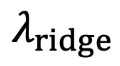
Figure 1 below displays the fraction of the time that the ( ,) combination performed best out of the sample. The right corner combination (1,0) represents runs with effectively no regularization and no decay. That combination performs best about 1/10^th of the time.

Figure 1
Frequency of Best-Performing Hyperparameter Combinations

This sample distribution suggests that 9/10ths of the time, some combination of decay weighting and regularization outperforms standard OLS.

Another prevalent combination is the left corner combination (1000, 0.1) where high regularization enables high decay (small ) forecasting. That combination performs best about 1/20^th of the time.

Lastly, a diagonal ripple in the implied surface of the image suggests that a higher regularization penalty facilitates forecasting with higher decay.

Conclusion and Further Study

The outperformance of non (1,0) combinations ofandis observable. The benefit of regularization may be more pronounced when more securities are used to forecast. Readers can perform their own investigation of this approach. Python code is available at this link.

Statements of fact and opinions expressed herein are those of the individual authors and are not necessarily those of the Society of Actuaries, the newsletter editors, or the respective authors’ employers.

David Romoff, MBA, MS, is a lecturer in the Enterprise Risk Management program at Columbia University. He can be reached at djr2132@columbia.edu.