Deep Learning in Risk Management: A Gentle Introduction
By Damon Levine
Risk Management, September 2022

In this article an artificial neural network (ANN) is applied to a real-world risk challenge. This high-level introduction to deep learning via ANNs uses only basic mathematical and statistical concepts. We begin with a familiar modeling approach, and then improve the method so it may “learn” to better fit the existing data and (hopefully) provide accurate projections for future values.
The data types are specified in the examples, but these methods work equally well across a very wide array of real-world problems and the specific context is irrelevant.
The only “requirement” is that the quantity of interest materially depends on a set of quantitative variables (e.g., historical data points) in a numerical way.
The Training Data Set
In many situations we have data for existing customers, and we want to use that data to assign a risk score to a potential customer.
In the example a bank has collected the following numerical fields for companies applying for a line of credit or loan:
- Acid test ratio: Current assets minus inventory divided by current liabilities.
- Balance sheet equity.
- Ratio of monthly net cashflow to monthly cash expenses.
- Financial health rating (e.g., S&P financial strength rating or equivalent private company rating).
- A score related to the company’s access to additional funds via credit lines or other sources.
Each of these will be scaled to be decimals in the range of [0,1], and we will refer to these explanatory variables as x1, x2, x3, x4, and x5, respectively. Suppose we know the risk rating, also in the range [0,1], which we view as correct for existing customers. We want to use this data to produce a risk rating for potential new business customers. Note that 1) the scaling may be done so that higher values correspond to higher or lower risk levels, as desired by the modeler, but this is not important for our purposes, and 2) the scaling is not a requirement for any of the techniques introduced.
As mentioned, we have the desired data on existing companies and know what risk scores they should have received. This will serve as our “training data” set and will calibrate our model.
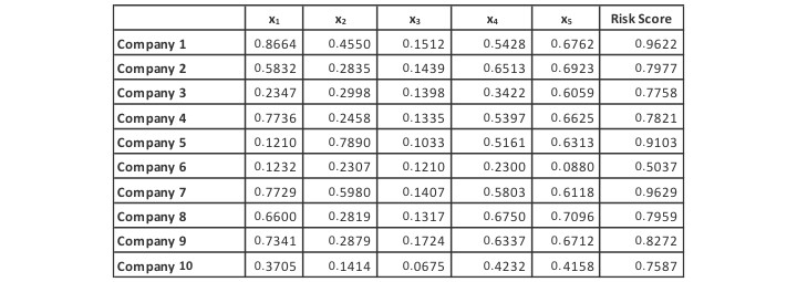
Our training data, consisting of the explanatory variables and their associated risk scores, is shown below in Exhibit I.
Exhibit I
The Training Data Set
A Linear Optimization
The goal is to find a model that assigns a risk score to any company based only on its five financial health variables, x1, x2, x3, x4, and x5. This model is “tuned” by using the data in Exhibit I. A simple approach is to assume the modeled risk score, f, is a linear combination of the input variables:
![]()
where the {wi} are “weights” (real constants) yet to be determined and we find the “best” possible weights. As a shorthand we can refer to this modeled risk score, for a company i, as f (company i).
We seek the weights that allow the function to perform well on the training data set. Our hope is that the function will also perform well on new companies which are not present in the training set.
We determine the values of the weights as those that minimize the sum of squared errors (SSE):
![]()
Where the summation is over i = 1 to 10, the entire training set.
The values of the weights that minimize the above-defined SSE for the linear function f are typically called regression coefficients, and the proposed optimization is nothing more than multiple linear regression (without constant term) on the training set.
We carry this out using Excel, leveraging the Solver add-in, and utilize the gradient descent method for optimization. Gradient descent essentially uses derivatives from calculus in order to iteratively improve the weights in terms of their impact on the SSE, or some other user-defined error or cost function. Some additional details on this approach appear later in this article.
The optimization indicates the best weights as follows:
![]()
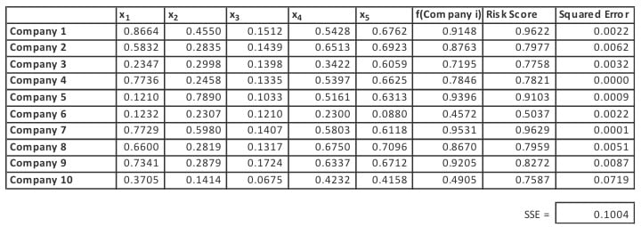
It performs well over the training set with the SSE equal to 0.1004 as shown in Exhibit II, below.
Exhibit II
Linear Model Performance on the Training Data
As mentioned, the model is fitted to the training data and then we look to its performance on that data as well as the test data, which is a set outside of the training data. In practice the test data may be a subset of data that was known at the time of the model fitting but purposely excluded from the training set. It also may be a data set obtained after such fitting. In either case it provides a litmus test of the fitted model in an out-of-sample environment. It is necessary that we know the actual value of the response variable for the test data which, in this case, is the Risk Score.
The test data is used gain confidence that the model will serve its intended purpose and serve as a strong predictor when used on data “in the wild”. If a model does not perform well on test data, then it cannot be regarded as a strong model, despite any positive results seen on the training data.
The performance over our test data, consisting of companies 11–15, is less impressive as shown below.
Exhibit III
Linear Model Performance on the Test Data
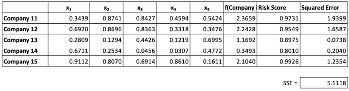
The model does not perform particularly well with a fairly large SSE of 5.1118. This points to at least two potential problems with linear models such as regression: 1) they may “overfit,” and 2) they cannot capture non-linear relationships between inputs and the output. The term overfit refers to a model that may be so “fine-tuned” to the training set that it performs poorly on the test set. Some would describe this as saying the model has “learned the noise” inherent in the training data.
A Non-linear Improvement
The previous optimization found weights, {wi} that produced the smallest SSE possible. The model “f” took as an input the explanatory variables for a given data point and its output was a linear combination as shown in Exhibit IV.
Exhibit IV
A Visual of the Linear Model
The weights may be chosen randomly or set equal to begin the optimization. For each data point in the training set, (x1, x2, x3, x4, x5), the modeled risk score, i.e., w1x1 + w2x2 + w3x3 + w4x4 + w5x5, is compared to its actual risk score to determine the error. The SSE (across all data points in the training set) is determined. The optimization then adjusts the weights and again computes the (improved) SSE. This continues until those weights producing the smallest possible SSE are determined.
As discussed, such a model cannot capture non-linear relationships between the {xi} for a company and the company’s actual risk score. Let us look at a different approach where we take the linear combination as an input to a new and non-linear function A.
The function A takes as its input u= f(x1, x2, x3, x4, x5), and its output is defined as 1/(1+e-u). In other words, A is the logistic function.
Exhibit V
Incorporating a Non-Linear Element in the Model
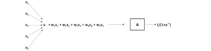
The optimal weights, {wi} are yet to be determined, and again, we minimize the SSE. Note that the above is simply a visual for a composition of functions: A(f(x1, x2, x3, x4, x5)).
The function A has an important role of creating non-linearity in the above diagram and is often called a “node.” The node takes a linear combination as its input and applies a non-linear function, typically called an “activation function,” to that value. In our case the input to node A is u= w1x1 + w2x2 + w3x3+ w4x4+ w5x5 and the output is 1/(1+e-u). The predicted risk score is this output of the node A. In practice, a constant term, called the “bias” is often used in the activation function, e.g., the output of the node could be 1/(1+e-u) +0.08, but we’ve assumed that the bias is zero in our example. Many other activation functions are common including the hyperbolic tangent and the rectified linear unit (“ReLU”) that is simply R(t) = max(0,t).
The optimal {wi} are determined and we now have a model where the input is a company’s data as (x1, x2, x3, x4, x5) and the output, i.e., predicted risk score, is 1/(1+e-u), where u = 1.3892x1 + 3.3936 x2 -7.0441 x3
-0.9820 x4 + 1.8822 x5.
This improved, non-linear, model has an SSE over the training set of 0.0123, better than the linear approach’s value of 0.1004. Also, we have gone from 5.1118 down to 2.4084 on the SSE for test data. For the sake of brevity, the granular numerical results are not shown here, but in our final optimization we’ll look at model performance in greater detail.
A Two-Layered Artificial Neural Network
As our last approach to the problem, we now use a slightly more complicated ANN to illustrate the structure of nodes, activation functions, and illustrate the deep learning concept of layers.
Exhibit VI shows our new ANN now has the following elements:
- Five weights that will be used in Node 1 and five other weights that are used for Node 2.
- Activation functions for Nodes 1 and 2 that are both the logistic function (again).
- Two additional weights used to form a linear combination of the outputs of Nodes 1 and 2.
- A third node, Node 3, takes the linear combination from (3) as an input.
- The output of Node 3, the logistic function applied to its input, is the modeled risk score.
Exhibit VI
A Depiction of the Artificial Neural Network
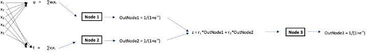
Note this is still a composition of functions where the input is (x1, x2, x3, x4, x5) and the output (as a result of the composition of functions) is 1/(1+e-z).
As before, we optimize the weights (now a total of 12 weights consisting of {wi}, {vj}, and the {rk} ) to minimize the SSE on the training data. The two Nodes, 1 and 2, form what we call the first “hidden layer” of the ANN, and Node 3 forms the second hidden layer. These hidden layers sit between the input and the output of the process. We now examine how this optimization performs on the training and test data.
Exhibit VII
Performance of the ANN on the Training Data
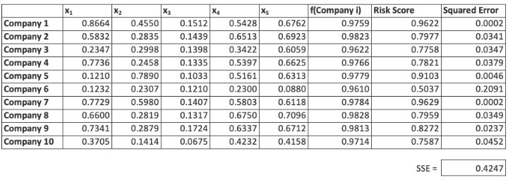
Exhibit VIII
Performance of the ANN on the Test Data
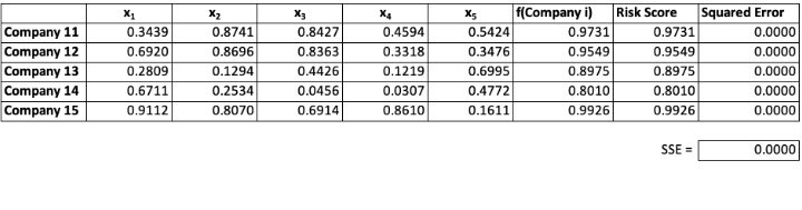
The ANN clearly shows a remarkedly better outcome for the test data set, while also fitting the training data well. This is exactly the type of result that we seek in real-world applications: The primary goal is predictive modeling, and the test data set is the proving ground. The SSE, which is very close to zero, points to the model’s success on the test data. Note that while the squared errors appear to be zero, this is due to rounding and they are actually non-zero.
There is, of course, a wide range of choices for the number of nodes, the number of weights, the choice of activation functions, and the number of hidden layers in the ANN.
Why the Optimization Works
We know from experience that linear regression is popular, in part, because its solution is mathematically tractable. It’s always easy to get the regression coefficients. Some who have attempted various optimizations in a business setting, possibly using Excel, probably have noticed that they often don’t work well. There is a tendency for the optimization procedure to get “stuck” in a local minimum that is only the minimum in a neighborhood, rather than the global minimum that we’re after.
As mentioned, we’ve utilized the gradient descent method in our optimizations. It is important to see that the outputs of the preceding diagrams are differentiable functions of the input values. As a result, the partial derivatives of the SSE with respect to each of the weights exist. This is a condition that makes gradient descent extremely powerful, especially when many input variables are being considered.
Furthermore, we have not imposed constraints on the weights such as lower bounds or arithmetic conditions on their sums or differences. This lack of constraints and the differentiability make gradient descent an effective tool. It’s important to realize we may still get stuck in a local minimum and not produce an optimal answer. What has been discovered is that when there is a “high” number of dimensions in the problem (i.e., high number of input variables), the local minimum problem often goes away. While the reasons behind this are not entirely understood, it is certainly a “happy” outcome and is a fundamental reason that these neural networks have had such tremendous success.
Of course, the gradient descent optimization can run into various problems including what is called the vanishing gradient problem. During each iteration of gradient descent, every weight receives an adjustment based on the partial derivative of the SSE (or other error or penalty function) with respect to the weight. In some cases, the partial derivatives for one or more weights start to approach zero before reaching an optimal solution, effectively preventing the weights from changing value. The ANN is then not able to “learn,” i.e., progress toward an optimal set of weights halts. There are, however, a large number of techniques to help mitigate this challenge.
Deep Learning in Risk Management
In Exhibit VI, we have two hidden layers of nodes between the input and the (final) output. In complicated applications such as image recognition the best solution is often one that has several layers. When the number of layers is high, e.g., 5–7, the ANN is said to be a “deep learning” network. So, the term “deep” in deep learning refers to a high number of hidden layers.
In many cases, including additional hidden layers in an ANN does not materially improve the model’s performance, but in many complex applications it proves worthwhile.
Applications of deep learning have seen tremendous success in areas including voice recognition, the games of Go and chess, and medical diagnosis. Opportunities abound in the field of risk management as well.
Risk management is often concerned with assigning a risk rating to something based on several known explanatory variables. When the underlying relationship is both numerical and complicated, deep learning may be the answer.
Suppose we are assigning an underwriting risk tier for health insurance applicants. We might consider explanatory variables including smoker status, health as determined by a doctor, age, gender, and other indicators that are associated with possible future claim behavior. As this is a complicated relationship, it may be useful to frame the problem as a deep learning optimization.
Another example can be found in third-party risk management. We may be interested in estimating the likelihood of a data breach at a third party. This can be viewed as a function of a company’s cyber security score (furnished by one of the many specialized platforms today), the type of data they touch, the time since their last breach, and other explanatory variables. This data can be used, via deep learning, to assign a score that estimates risk of breach, reflecting both probability and potential dollar impact.
The primary human input into ANNs is the articulation of the explanatory variables that influence the unknown metric of interest. It is clear there the next example of a significant ANN success is just around the corner. It is, however, harder to predict in just what areas these will come next.
Statements of fact and opinions expressed herein are those of the individual authors and are not necessarily those of the Society of Actuaries, the newsletter editors, or the respective authors’ employers.
Damon Levine, CFA, ARM, CRCMP is a risk consultant specializing in banking and insurance ERM. He can be reached at DamonLevineCFA@gmail.com.