Confusing the Matrix: The Last Part
By Ryan LaMar Holt and Ryan Shubert
Product Matters!, November 2024

Welcome to the finale! A couple years ago the “Confusing the Matrix” series launched on a journey to document the assumptions and methods actuaries were using to estimate the mortality impact associated with less invasive underwriting practices. With a third and final installment, we hope to join the ranks of other excellent trilogies with actuarial adjacent names such as “Back to the Future,” “The Matrix,” and of course “Die Hard.” In this edition we will look at understanding the volatility of mortality impacts estimated from an audit sample. We will also demonstrate how to break the mortality impact estimate into component pieces. The examples shown in this article assume a general understanding of how mortality impacts are estimated from an underwriting audit sample. If the reader needs any background on this topic, the prior two “Confusing the Matrix” articles provide a good baseline. Throughout the article we will also use the same sample data that was presented in “Confusing the Matrix: Part Deux.”
Sample Data
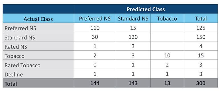
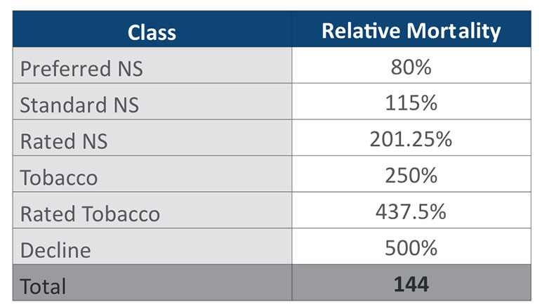
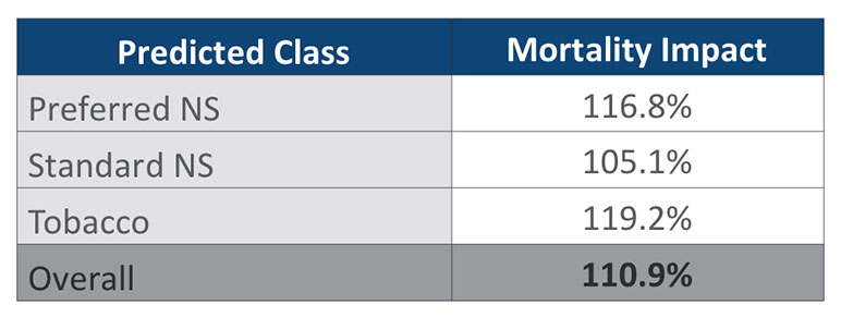
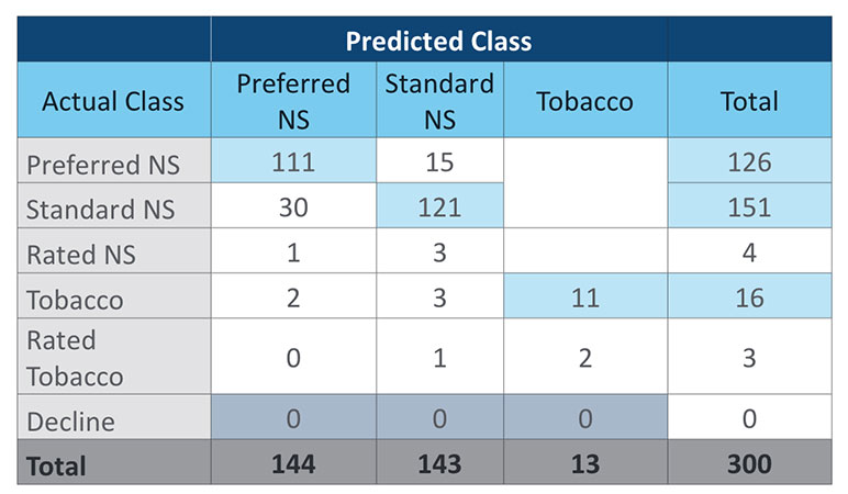
For the benefit of the reader, we will restate the sample data that will be used for the examples in this article. Table 1 is a simplified confusion matrix with fabricated audit data. Table 2 provides the relative mortality assumptions that will be used in the duration 1 mortality impact calculation. For simplicity, this article will focus on a duration 1 mortality impact calculation rather than presenting all the different methods explored in the prior article. Table 3 shows the duration 1 mortality impact overall and by risk class for the sample data.
Table 1
Table 2
Table 3
Volatility
Measuring the volatility of the estimated mortality impact from an audit sample can get very technical rather quickly. We are going to gloss over some of the more technical aspects and assume that the reader can access the appropriate statistical expertise if further understanding is needed. Put simply, there is no closed form solution to calculate the variance of our mortality impact estimate. The estimate is a ratio of two random variables (pre- and post-audit results) regardless of the method used to calculate the impact. While there is no closed form solution for the variance of the ratio of two random variables, we can estimate the variance using either a Taylor Series expansion (if certain assumptions are met) or by bootstrapping. For this article, we will focus on the bootstrap method, as it can be applied in all situations and the data created provides a nice visual of the estimated sampling distribution.
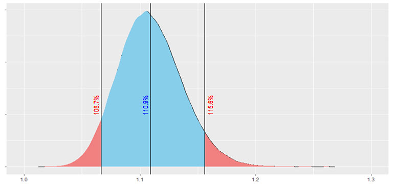
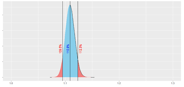
Jumping right into that, Figure 1 illustrates a bootstrapped sampling distribution using the sample data presented in Table 1 which has a sample size of 300. Figure 2 presents a bootstrapped sampling distribution using altered data from Table 1, with all the counts multiplied by 10 to create a sample size of 3,000. Both cases used 100,000 iterations to create the bootstrapped sampling distribution. A non-parametric 90% confidence interval is also shown in both figures, which simply selects the 5th percentile and 95th percentile from the bootstrapped sample mortality impacts.
Figure 1
Figure 2
There are two immediate observations from these figures. First off, hopefully it is painfully obvious to the reader that the larger our sample size is, the less volatility we will have around the estimated mortality impact.
The second observation is that the sampling distribution is slightly skewed, with a steeper tail on the left-hand side and a longer tail on the right-hand side. This makes sense for our sample, and for most audit samples of this type, because there is almost always more downside risk (higher mortality impact) than upside risk (lower mortality impact). This is because there are fewer opportunities for reverse misclassification (when a preferred risk is offered a risk class worse than preferred) compared to opportunities for detrimental forms of misclassification. Essentially, the probability that a bootstrapped sample will produce a worse result than the baseline estimate is larger than the probability that a bootstrapped sample will produce a better result than the baseline. This leads to the longer tail to the right of the distribution.
Understanding the volatility associated with the point estimate for mortality impact can then help inform decision making around mortality assumptions. For example, if we had assumed an 8% mortality impact in pricing for our less invasive underwriting program, at a sample size of 300 we could say that our assumed pricing impact is not out of line with what we are observing from the audit results. However, at a sample size of 3,000 we would conclude that the estimated mortality impact from the audit now exceeds our priced for mortality impact.
The bootstrap can also provide a way to determine if there are statistically significant differences between groups within an audit sample, such as results by sex, issue age, or face amount. In the January 2024 issue of The Actuary, the article “Accelerated Underwriting Analysis,” authored by Taylor Pickett and Christine Kachelmuss, presented many differences that have been observed among these various groups within actual audit results. Understanding how significant these differences are for a specific program can help determine if a different expectation is needed across different policyholder attributes.
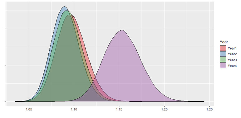
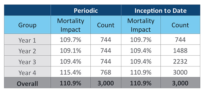
Comparing results by issue year or program era can also provide valuable insights. Figure 3 takes the same data used in Figure 2, but I have split it into four issue years with approximately similar sample sizes and intentionally skewed the results of the fourth year. Table 4 summarizes the mortality impact and sample size for each year.
Figure 3
Table 4
A key takeaway from Figure 3 and Table 4 is that inception-to-date results can be misleading. Given that more data leads to less volatility around estimated mortality impact, it can be tempting to use all the data available all the time. In this case, if we only look at the inception-to-date results it looks like a small increase to mortality impact in Year 4. The weight of the prior three years of consistent results dulls the impact of the poor result in Year 4. If there is a known change to a program, there is even greater need for partitioning audit results by era. Introducing a new model, significant changes to underwriting rules, starting sales with a new distribution partner. These could all lead to different outcomes and are worth giving up a credible audit sample in exchange for a relevant audit sample.
A secondary takeaway from Figure 3 and Table 4 is that the bootstrap can help determine when a new era or issue year has deviated significantly from prior results. In Figure 3, Year 4 is clearly increased from the prior three years. But we still see some overlap in the tails of all four years. It’s possible that Year 4 is just an unlucky sample. If you were to use a strict p-value of 0.01, you would not be able to state that higher outcome in Year 4 is a statistically significant difference. While there certainly is a need investigate the results from Year 4, the bootstrap can help put some statistical rigor around decisions related to the estimated mortality impact.
Considerations for Bootstrapping
The estimates from a bootstrap are only as good as the data you have available. The bootstrapped samples do not anticipate any possible changes to the audit sample in the future. If you have not observed any declines in your audit sample, then the volatility projected by the bootstrap anticipates that there will never be any declines in your audit sample. As a result, a small sample without any observed low frequency/high severity misses may present an optimistic view of the estimated volatility of the sample.
To address the concern of missing observations, some in the industry have proposed using additive smoothing. This technique adds in observations for each cell of the matrix to try and account for possible missing observations. How much to add is somewhat subjective and should be sensitivity tested if this approach is used. Another approach could be to add in a prior expectation for cells within the confusion matrix that have no observations. The expected distribution could come from a retrospective study or from observations in industry studies. Lastly, one could simply not adjust at all and recognize that this is a shortcoming of the bootstrap when interpreting results for small sample sizes.
As an audit sample grows, missing values become less frequent and smoothing becomes less relevant. In fact, missing or null values in a confusion matrix when an audit sample is substantial could be interesting observations in and of themselves. Actuaries, underwriters, and data scientists involved in analyzing audit data should collaborate in determining which approach best fits their needs.
Impact Contribution
The estimate of mortality impact is a valuable tool in determining if mortality for less invasive underwriting programs is performing as expected. If we dig deeper into the mortality impact, it can also be a useful tool for identifying specific areas for improvement in these underwriting programs. The level of detail you can achieve depends on the data collected when an underwriter reviews an audit. The most granular level would be able to identify what impairment caused a case to be misclassified (i.e., liver function, cholesterol, specific personal medical history, and so on).
Table 5
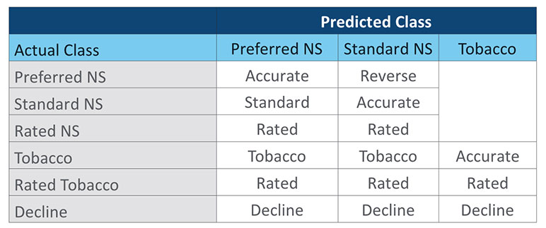
If this granular level of detail has not been captured, a more generic type of misclassification can be categorized as shown in Table 5. There is some judgement in assigning these categories. Note that cases with an Actual Class of Rated Tobacco and a Predicted Nonsmoker class are both a rated miss and tobacco miss. For this exercise we have categorized them in the Rated group. Others might want to count them in the Tobacco category. A third option could be to have a Rated Tobacco category. For calculation purposes it is important that each category is mutually exclusive. Additional consideration is needed when classifying misses at the impairment level, where there could often be multiple reasons for a misclassification, such as both build and blood pressure.
With each observation of the confusion matrix assigned to a type of misclassification, we can then determine how much of the mortality impact is driven by that group of misclassifications. We will walk through this calculation at a rudimentary level to help illustrate the process. The reader is advised that there are more efficient ways to calculate this in practice. To start, we assume that each observation for a given group was accurately classified. Using the decline category from our sample data as an example, the three declines can be relocated to the appropriate accurate class as shown in Table 6.
Table 6
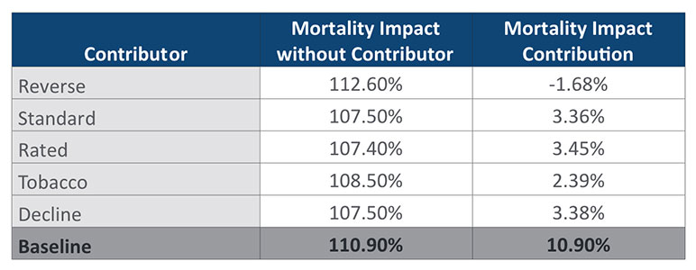
Recalculating the duration 1 mortality impact with declines shifted to accurate cases we get a new estimate of 107.5%. This is a reduction of 3.4% points from the original estimate of 110.9%. Put another way, 3.4% of the 10.9% overall mortality impact comes from declines alone. If you repeat this exercise with all the other categories, you end up with the table of mortality impact contributions shown in Table 7.
Table 7
Determining each group’s contribution to mortality impact provides value by identifying the largest sources of mortality impact for an audit sample. For the sample data used here, results are close to evenly split between the three largest contributors: Standard, Rated, and Decline misclassifications. When calculating impact contributions this way, the sum of the different contributions will always add up to the total estimate of mortality impact.
Knowing the largest drivers of mortality impact can help focus your efforts on areas where taking action would provide the most benefit. If you have identified the specific impairments that were the main reason for misclassification, you can apply this approach in determining the contribution to mortality impact for specific impairment groups. If you do not currently track these reasons, you are missing out on the ability to pinpoint problem areas with your less invasive underwriting, as well as the ability to prioritize what impairments are costing you the most.
Conclusion
Understanding the volatility associated with audit samples, as well as breaking out the different contributors to estimated mortality impact are vital tools in helping actuaries and underwriters make informed decisions about less invasive underwriting programs. As life insurance underwriting continues to evolve, actuaries and underwriters will need to work collaboratively to understand how these changes impact future expectations. Auditing new underwriting programs, particularly those that have pulled back from the detailed medical information that has formed the baseline of our mortality experience for the last three decades, has been vital to providing insights into how future mortality experience will emerge. With credible mortality experience still out of reach for newer underwriting paradigms and the continual evolution of underwriting practices, it is likely that the assumptions and methods documented in this article series will be needed and beneficial to the profession for many years to come.
Statements of fact and opinions expressed herein are those of the individual authors and are not necessarily those of the Society of Actuaries, the editors, or the respective authors’ employers.
Ryan LaMar Holt, FSA, is a vice president and actuary in RGA’s U.S. Individual Life division. He can be reached at ryan.holt@rgare.com.
Ryan Shubert, FSA, is an actuary on RGA’s U.S. Individual Life assumption team. He can be reached at rshubert@rgare.com.

