Challenges of Managing Interest Rate Risk: Part 3—How to get the Most Insight out of a Company’s Assets and Liabilities
By Dariush Akhtari
Risk Management, June 2024

In the mid-‘80s Tom Ho introduced the concept of key rate metrics to address the fact that interest rates do not move in parallel across the yield curve; today most use the spot curve as opposed to the yield curve. If one considers the impact of each tenor’s rate change to the value, then the sum of the impacts across all tenors should be the impact of rate change across the entire curve and this would eliminate the issue of rates not moving in parallel. So, one would calculate the ALM metrics only when the 10-year rate was shifted up and down by some basis point; the 10-year key rate metric. But this meant that one needed to calculate 30 key durations and convexities to capture the impact of the full rate change across a 30-year spot curve. Others noted that rates in some periods do move reasonably flat and instead of using every tenor, one could group tenors that have rates that move closer to parallel. This would reduce the calculation time with little loss of accuracy. The splits used by many are rates in tenors less than two years, two to five, five to 10, 10 to 20, and 20 to 30. Note that this split is not unique as others have used different splits such as tenors zero to two, two to five, five to seven, seven to 10, and 10 to 30, or other splits. Generally, the naming of the key rate is tied to the ending period. For example, metrics for a zero to two period are called a two-year key rate and for two to five, it is called a five-year key rate. While for the calculation of duration and convexity the entire curve is shifted up or down by some basis points, for the calculation of key-rate duration and key rate convexity only the tenors affecting the key rate are shifted. For example, for two-year key rate metrics only tenors less than two years are shifted and for five-year key rate metrics, rates for tenors two to five are shifted. An example of how the shift in rates is done is depicted later in this article in Appendix 1, Table A1.1.
Early on, the above shifts were used however, to capture some element of interaction between neighboring periods, the shift in rates were linearly graded between the neighboring key rate periods. An example of how the shift in rates is applied is depicted later in this article in Appendix 1, Table A2.1. Note that in either approach the sum of the shifts in the key rates add up to the flat shift to the curve.
Formulae and Definitions
In the below, “V” represents the present values of what is being discounted (generally cash flows or profits). A subscript of “+”, “-“, or “0,” is added to reflect whether the shift is positive, negative, or no shift respectively. The “++” and “--” subscripts mean twice the shift size has been applied. The letter “k” is added to “V” to reflect that the rate shift is applied to key rates k.
The change in the discounted values when a positive shift (+h) is applied to the entire curve is denoted by “P” for positive shift and when the shift is negative (-h), it is denoted by “M” for “Minus.” When a “k” is added to “P” or “M” it denotes that the shift is only applied to the portion of the curve covered by key rate k.
Mkh = Vk- – V0 → Vk- = Mkh + V0 Note: Mkh for an option-free bond is positive.
Mh = V- – V0 → V- = Mh + V0 Note: Mh for an option-free bond is positive.
Pkh = Vk+ – V 0 → Vk+ = Pkh + V0 Note: Pkh for an option-free bond is negative.
Ph = V+ – V 0 → V+ = Ph + V0 Note: Ph for an option-free bond is negative.
Mk2h = Vk- - – V0 → Vk- - = Mk2h + V0 Note: Mk2h for an option-free bond is positive.
M2h = V- - – V0 → V- - = M2h + V0 Note: M2h for an option-free bond is positive.
Pk2h = Vk+ + – V0 → Vk+ + = Pk2h + V0 Note: Pk2h for an option-free bond is negative.
P2h = V+ + – V0 → V+ + = P2h + V0 Note: P2h for an option-free bond is negative.
Note that while in the calculation of P, M, and V, the rate shift, h, is say +0.1% or 10bps, in the below h is the value of the shift in basis points (bps) meaning using h = 10.
DV01 = (V+ – V-) / (2 * h) = (Ph – Mh) / (2 * h)
Note: DV01 for an option-free bond is negative (as rates increase, value decreases).
CV01 = (V- + V+ – 2 * V0) / h2 = (Mh + Ph) / h2
Note: CV01 for an option-free bond is positive.
Speed01 = [V+ + − V- - – 2 * (V+ − V-)] / (2 * h3) → Speed01 = [P2h – M2h – 2 * (Ph – Mh)] / (2 * h3) →
Speed01 = (P2h – M2h) / (2 * h3) – 2 * DV01 / h2
Note, after a parallel change of k bps (positive or negative) to the curve:
VAfter = VBefore + DV01 * k + CV01 / 2 * k2 + Speed01 / 6 * k3 →
∆V = DV01 * k + CV01 / 2 * k2 + Speed01 / 6 * k3
DV01After = DV01Before + CV01Before * k + Speed01Before / 2 * k2 →
∆DV01 = CV01Before * k + Speed01Before / 2 * k2
CV01After = CV01Before + Speed01Before * k →
∆CV01 = Speed01Before * k
For the equivalent key rate calculation of the above metrics, denote each metric by adding “KRk” in front of it to indicate that it is the key rate k that is being calculated additionally, replace P, M and V with Pk, Mk, and Vk respectively as in:
KRkDV01 = (Vk+ – Vk-) / (2 * h) = (Pkh – Mkh) / (2 * h) where “KRkDV01” refers to DV01 for key rate k.
Adjustments to the above Calculated Formulae
Since rate shifts in the calculation of Pkhs add up to a parallel shift to the entire curve, one would expect that the sum of Pkhs adds up to Ph. Similarly, the expectation is that the sum of Mkhs adds up to Mh. However, while the sum of key rate metrics is close to the metrics when the shift is applied to the entire curve, they are not identical. This is due to the fact that there are interactions between the key rates that impact the value (cross key rate or cross Greeks). Note that this problem exacerbates when shift size is increased, as discussed in Part 2, due to inflection points.
In practice, a number of approaches are applied to correct for this. The first is to ignore the differences, meaning to ignore any cross key rate impact. This is the worst approach.
The second is to scale KRkDV01, KRkCV01, and KRkSpeed01 to match their respective metrics in the parallel shift, namely DV01, CV01, and Speed01 respectively, to reflect the impact of cross key rate on each metric. This, too, is not a good approach as it suggests applying different scales to Pks and Mks in the calculation of these metrics. Note that DV01, CV01, and Speed01 are byproducts of Pks and Mks. This means finding a different scale, Sm, for each KRMetric as below and then using the scaled KRMetric for approximations.
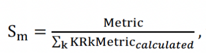 then KRMetricused = Sm * KRMetriccalculated where Metric refers to DV01, CV01, and Speed01.
A third approach is to apply a scale to Pks to match P and a different scale to Mks to match M. Of the three approaches, this is more appropriate. However, blindly applying scaling to calculated metrics is flawed. In the next article in this series, I will highlight how drastic such scales would be. When the scale is close to 100% (say 95% to 105%), the impact might not be material. However, there are situations where one or both scales could be in excess of 300% or below 30%. This means finding a scale, Sm, for each KRValue as below and then using the scaled KRValue in the calculation of KRMetrics.
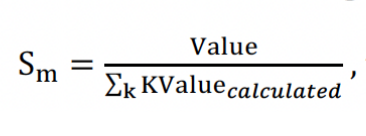 , then KValueused = Sm * KValuecalculated where Value refers to P, and M.
A fourth approach is to reflect every cross key rate impact (see Appendix 3 later in this article for how to calculate these). This approach, while more appropriate since it captures the impact of every key rate on another, requires n times more runs where n is the number of key rates. Note that this approach requires capturing all the combinations of the up shifts and down shifts of every key rate with other key rates, thus increasing runtime. In particular, when using stochastic models for liabilities in insurance companies, the sheer number of runs needed for this approach, makes it almost impossible to use. In fact, the need for these additional runs is one reason that the scaling approach is used, meaning scaling is used to reflect the impact of cross key rates in the calculated metrics.
New Proposed Approach
To avoid the extra runs and avoid unreasonably high or low scaling factors, yet to be able to capture the cross Greeks without the need for scaling, I developed the following approach, which I call cumulative key rate. Instead of the normal key rate shifts, one first captures a cumulative key rate shift (see Appendix 2). The shift in rates in the periods (used for the calculation of cumulative key rates) is the sum of the shift in rates in all the periods used in the prior key rates. If we assume the key rates being used are two, five, 10, 20 and 30 years, then the two-year cumulative KR shift is the same as the two-year KR shift in rates. However, the five-year cumulative KR shift is the sum of two-year and five-year KR shift in rates for periods affecting both two- and five-year key rates. Similarly, the 10-year cumulative KR shift is the sum of the two-year, five-year and 10-year KR shift in rates for periods affecting both two-, five- and 10-year key rates. This means that the 30-year cumulative KR shift in rates (the last key rate) is the sum of the two-year, five-year, 10-year, 20-year and 30-year KR shift in rates, which will actually equal to a flat shift to the entire curve. To calculate the KR values from the cumulative KR up/down shift in rates, one takes the difference of the value generated in the current cumulative KR up/down shift in rates less the value created by the immediately prior cumulative KR up/down shift in rates. This approach, incorporates the cross Greek between two-year and five-year KRs in the five-year KR. Similarly, the cross Greek for two-year, five-year, and 10-year KRs is incorporated in the 10-year KR. In essence, all the cross Greeks are included in the calculated KRs and no scaling would be necessary. Since there is no scaling applied, the sum of KRkDV01, KRkCV01, and KRkSpeed01 equal DV01, CV01, and Speed01 respectively. This is closer to reality as closer key rates should incorporate more of the cross Greek whereas the scaling suggests that the cross Greek is proportional to the value rather than the proximity of the rates.
Formulaically, for the up and down shifts we have:
![]() where CKRates are rates used in shifted value calculations, and
where CKRates are rates used in shifted value calculations, and ![]() where CKValues are the shifted values created when cumulative shifted rates are used (value refers to P and M as above).
where CKValues are the shifted values created when cumulative shifted rates are used (value refers to P and M as above).
In the following parts of this article series, I will present how this approach provides more stable results, compared to the above approaches, with fewer runs.
Statements of fact and opinions expressed herein are those of the individual authors and are not necessarily those of the Society of Actuaries, the newsletter editors, or the respective authors’ employers.
Dariush Akhtari, FSA, FCIA, MAAA, is chief actuary at Converge RE. He can be contacted at dakhtari@converge-re.com.