Analysis of 2020 S&P Equity Returns and the Importance for Actuaries
By Zak Fischer
The Modeling Platform, July 2021

Overview
Most would agree 2020 was a year like no other. Between the COVID-19 pandemic, a heated U.S. political election, BREXIT, Tiger King, and more, 2020 was a unique year that many of us will always remember, for better or worse. While the world itself was quite strange in 2020, was stock market performance in 2020 also unusual? In this article, we will explore equity market performance in 2020 using the S&P 500 Total Return Index (SP500TR).
During March 2020, COVID-19 concerns escalated in the U.S. and lockdown measures were announced. Market returns in March 2020 were quite extreme and choppy, alternating between days of huge gains and losses. March 16th was a particularly extreme market selloff. It was the largest point drop ever recorded for the S&P 500. Stocks dropped significantly after heightened concerns that the pandemic could have longer-lasting impacts than initially thought. On the other hand, March 13th and 24th were the two highest point increases ever recorded for the S&P 500. March was a time of heightened volatility with both sharp increases and decreases in equity markets, as seen in Table 1.
Table 1
Analysis of Extreme Market Movements in March 2020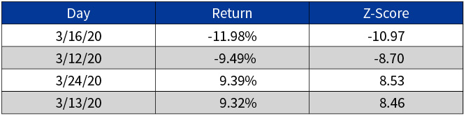
The Z-scores shown in the Table 1 are extremely large in magnitude. For a normal distribution, 68 percent of observations are within one standard deviation, 95 percent within two standard deviations, and 99.7 percent within three standard deviations. The odds of a Z-score with a magnitude above 8-10 is extremely small, less than 1-in-100 trillion.
As investors prepare for the future, it is important to understand whether these volatility surges and sharp movements are understood and captured by commonly used models. For example, the popular Black-Scholes model assumes that stock price returns are normally distributed and stock price levels are lognormally distributed. The large Z-scores in Table 1 point out that the commonly used normal distribution assumption is lacking in its ability to explain tail events. Tail events are often of great importance for a variety of actuarial applications, and so this is particularly important for actuaries to understand.
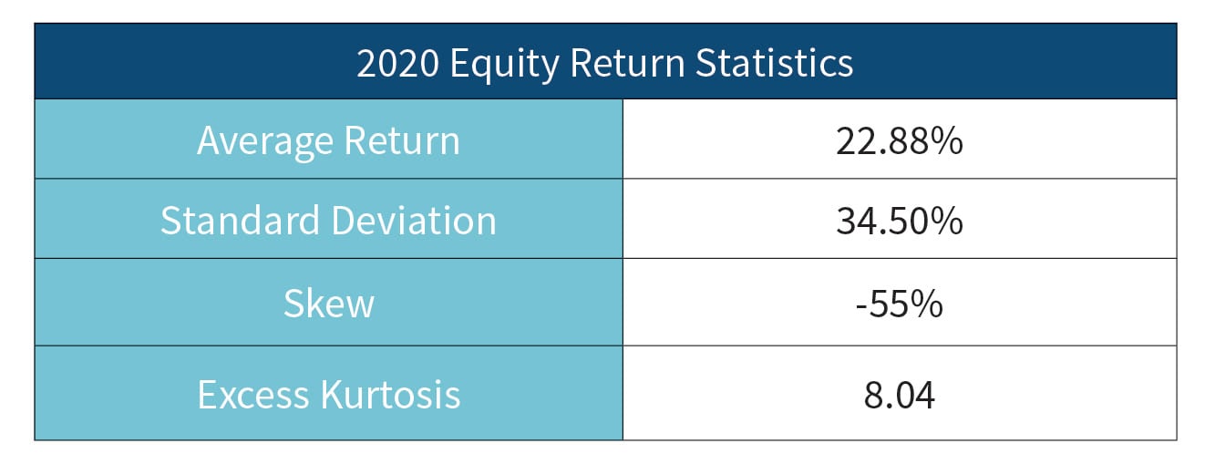
Next, summary statistics are computed below. Note that the excess kurtosis was quite large at 8.04. Recall that a normal distribution has kurtosis of three and excess kurtosis of zero. Therefore, 2020 equity returns, with an excess kurtosis of 8.04, had substantially heavier tails than a normal distribution.
Table 2
Summary Statistics from 2020 Equity Returns
Model Comparison
This section explores modeling equity returns using five different distribution assumptions: Normal, Student’s t, Regime Switching Lognormal (2 Regime), Extreme Value Theory and Poisson Jump.[1] Two different tests are performed on each of the distribution assumptions:
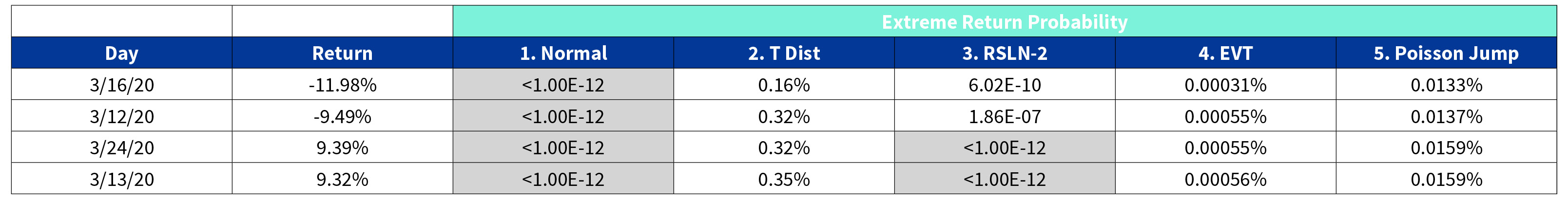
1. Extreme Return Probability—Ideally, models should assign reasonable probabilities to the extreme returns seen in March 2020. For example, a probability of less than 1-in-1 trillion (marked using “<1.00E-12” in Table 3) is unreasonable. Therefore, based on Table 3, the normal distribution is unable to explain the extreme market movements from March 2020. Additionally, the RSLN-2 model is unable to explain large market surges.
Table 3
Extreme Return Probabilities
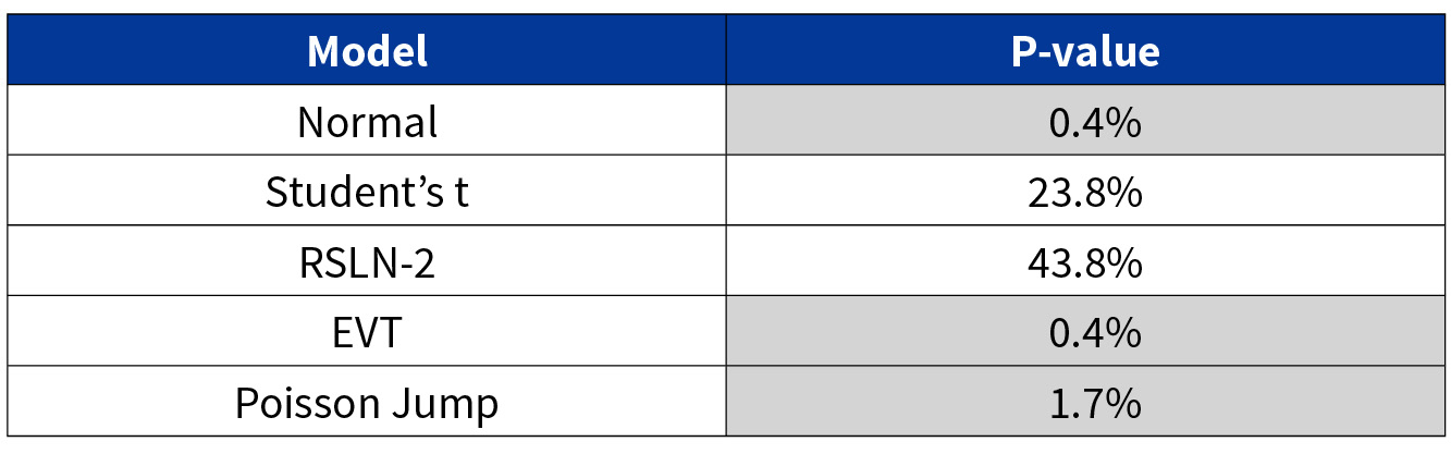
2. Non-Parametric Kolmogorov-Smirnov Test—Next, the Kolmogorov-Smirnov test is run to determine if the models can explain the full distribution of 2020 equity returns (and not just extreme returns). A small p-value indicates a poor fit and that the model behaves statistically significantly different than 2020 equity returns. The RSLN-2 are Student's t models are the only models that fail to reject the null at a 5 percent confidence level, indicating that they are potentially overall the strongest of the models at explaining 2020 equity returns.
Table 4
P-Values
The results of the two tests are summarized in Table 5.
Table 5
Results Summary
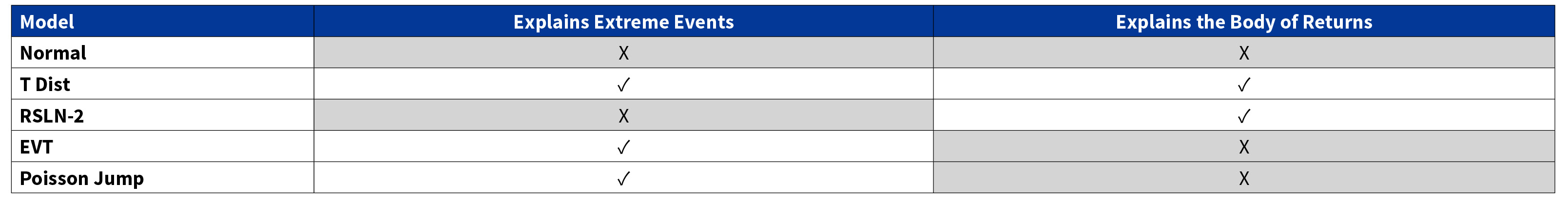
Note that the Student’s t distribution is the only model that is able to explain both extreme events and the body of returns. However, this does not imply it is a perfect model. Each of the five different models has advantages and disadvantages as seen in Table 6.
Table 6
Advantages and Disadvantages of Each Model Type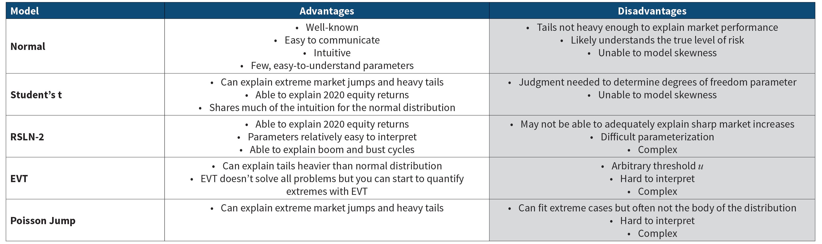
Mild Versus Wild Randomness
Despite its disadvantages, the normal distribution is still an enormously popular tool that has gained recognition in a large number of fields:
“Conventional studies of uncertainty, whether in statistics, economics, finance, or social science, have largely stayed close to the so-called bell curve, a symmetrical graph that represents a probability distribution. Used to great effect to describe errors in astronomical measurement by the 19th-century mathematician Carl Friedrich Gauss, the bell curve, or Gaussian model, has since pervaded our business and scientific culture, and terms like sigma, variance, standard deviation, correlation, R-square, and Sharpe ratio are all directly linked to it. Neoclassical finance and portfolio theory are completely grounded in it.” (Diebold, 86)
Diebold describes that the world in fact has two kinds of randomness: “mild randomness” and “wild randomness.” Quantities that follow the normal distribution or other distributions without large deviances have mild randomness. Wild randomness, on the other hand, occurs when “a single observation or particular number can impact the total in a disproportionate way.” Variables such as height, weight and IQ all obey mild randomness. In contrast, financial quantities such as wealth and stock returns exhibit wild randomness. As an example, you would not expect any adult to be 100 times taller than another adult. Yet, many people such as Bill Gates are easily more than 100 times wealthier than the vast majority of adults. While the normal distribution is often adequate to describe mild randomness, the normal distribution does not have sufficiently heavy tails to describe wild randomness. Therefore, those that rely on the normal distribution, such as those using the Black-Scholes model for stock returns, need to understand and appreciate the model shortcomings and associated risks.
The fact that the normal distribution does not adequately predict rare events is a well-known phenomenon in many areas, including financial markets. The prior analysis of extreme 2020 equity returns provides a remainder that this is still the case. Nicholas Taleb, a former options trader, acknowledges this idea in his book The Black Swan: The Impact of the Highly Improbable. His book emphasizes our blindness with respect to randomness, particularly large deviations. Taleb emphasizes that attempting to predict rare, “Black Swan” events is often futile; instead, focus on building robustness to extreme events. This means that firms should both be prepared to take full benefit of positive events, but also have adequate resources to prevent failure under conditions of adverse change. This closely coincides with the ideas of stress testing and contingency planning. In other words, none of the distributions from Section B are perfect. Qualitative methods should be employed to supplement any quantitative modeling to ensure firms have a broad understanding of their risk exposures.
Importance for Actuaries
Practitioners already know that the normal distribution is an imperfect distribution assumption and does not truly reflect the behavior of the stock market. The Black-Scholes options pricing model assumes that stock price returns follow a normal distribution. However, stock price returns have a much heavier tail than the normal distribution (i.e., leptokurtic), and so directly applying the Black-Scholes framework will often underprice options that are far out of the money. This is due to the fact that the normal distribution gives nearly no weight to Z-scores above eight, but these extreme market returns are in fact observed and have material financial implications. Those relying on the normal distribution or Black-Scholes model need to understand the shortcomings of these models and that they may underestimate tail risk. Alternatives to the Black-Scholes model could be considered, such as stochastic volatility models or models that consider smile/smirks in volatility surfaces.
Actuaries can supplement risk analysis with stress testing and scenario analysis to more rigorously quantify the impact and prepare for extreme events. There is no perfect-distribution assumption: common sense, expert judgment and supplemental methods such as sensitivity tests should all be used when modeling.
Perhaps the only certainty about markets is that they will continue to remain uncertain. Financial planning should consider the reality that market turbulence may persist.
Conclusion
March 2020 had four days with returns over an absolute magnitude of 9 percent. This corresponds to a Z-score when using a normal distribution of over eight, which gives an unreasonably small probability of extreme returns. Equity returns in 2020 had heavy tails with an excess kurtosis of over eight, indicating much heavier tails than a normal distribution.
The Poisson Jump, EVT, and Student's t models are able to explain extreme returns well from a probabilistic perspective. However, while the Poisson Jump can model thicker tails, it may sacrifice substantial fit in the body of the distribution and not perform well to explain typical cases. The RSLN-2 and Student's t distributions were the strongest of the models at explaining 2020 equity returns and were the only distributions statistically able to explain 2020 market performance when using the Kolmogorov-Smirnov test.
The Student's t distribution was the only model to pass the Kolmogorov-Smirnov test and have reasonable extreme return probabilities. Therefore, using these two tests as the criteria, the Student's t distribution was the best of the models at explaining 2020 equity returns. Of course, this does not imply it is a “perfect” model; for example, it cannot capture negative skew.
No one particular model is always better than any other. There are advantages and disadvantages of each equity model considered in this paper. Analyzing risk under multiple different distribution assumptions and parameterizations, as well as supplementing with qualitative analysis, may give a more holistic picture of risk.
Statements of fact and opinions expressed herein are those of the individual authors and are not necessarily those of the Society of Actuaries, the newsletter editors, or the respective authors’ employers.
Zak Fischer, FSA, CERA, is an instructor for The Infinite Actuary (TIA). He can be contacted at zak@theinfiniteactuary.com.