Economic Scenario Generators, Part III: In-depth ESG Case Study—Academy Interest Rate Generator
By Rahat Jain, Dean Kerr and Matthew Zhang
The Modeling Platform, July 2021

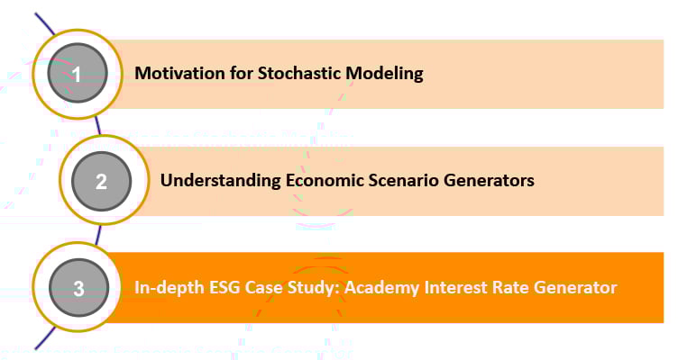
This article is the final installment of our three-part series on economic scenario generators (ESGs). Part I and II were published in the November 2019 [Economic Scenario Generators, Part I: Motivation For Stochastic Modeling (soa.org)] and August 2020 [Economic Scenario Generators, Part II: Understanding Economic Scenario Generators (soa.org)] issues of The Modeling Platform. Part III contextualizes the framework for selecting, building, and validating ESGs and focuses on the Academy Interest Rate Generator (AIRG), the most commonly used real-world ESG for US actuaries.
Figure 1
ESG Three-part Series Structure
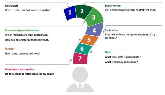
Jointly produced by the American Academy of Actuaries (the Academy) and Society of Actuaries (SOA), the AIRG applies to modern US regulatory reserving and capital regimes, such as VM-20 and VM-21, but has seen use since C3P2 and AG43. The ESG comes in a freely available and user-friendly Excel format, which requires minimal user input; i.e., the details lie “behind the scenes.” This article will cover the seven-step process described in Part II and shown in Figure 2 below, to elaborate on the specifics of the AIRG.
Figure 2
Key Factors When Making Decisions With ESGs
Risk Factors
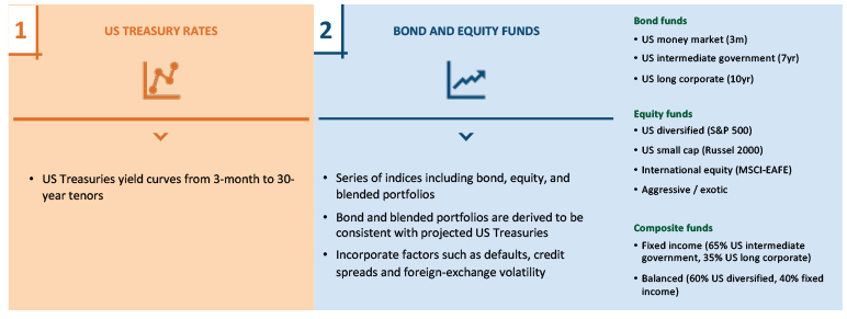
The AIRG models two risk factors: US Treasury rates and series of bond and equity fund returns, as described in Figure 3.
Figure 3
AIRG Modeled Risk-factors
While a two-risk factor ERG supports out-of-the-box modeling for commonly available investment options, the AIRG is considered a simple ESG, and has some notable limitations:
- Non-US economies are not directly modeled.
- Factors such as defaults, credit spreads, inflation, dividends, and foreign exchange volatility are buried within parameters and not explicitly modeled.
- Only aggregate fund indices are available.
- Mappings must be applied from actual investment options to the funds provided by the AIRG.
While the simplicity of the AIRG may be suitable for its valuation-focused use cases, its capabilities may be limiting for certain use cases and there is little room to customize or re-parameterize the model.
Scenario Type
The AIRG produces real-world scenarios intended to simulate the future in a “realistic” way by generating plausible outcomes aligned to past observed experience. This currently includes exhibiting characteristics such as a higher expected risk-adjusted return on riskier assets, volatility clustering, and a rising yield curve. The primary use case is to support US capital and reserve standards, where tail risk across real-world outcomes is the key focus.
The AIRG does not have risk-neutral capabilities or apply any form of market calibration, and therefore is not appropriate for use in market-consistent valuation.
Process and Parameterization
The AIRG models its two risk factors through fairly unique approaches, which will be discussed separately.
Interest Rates
Constant parameter models were determined as inadequate in simulating history, in particular because they tend to inadequately demonstrate a fat tail and extreme peaks, which are both key considerations for scenarios supporting reserving and capital calculations.
Figure 4
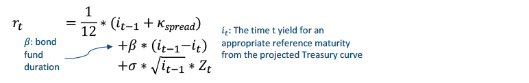
Stochastic Log Volatility Interest Rate Model
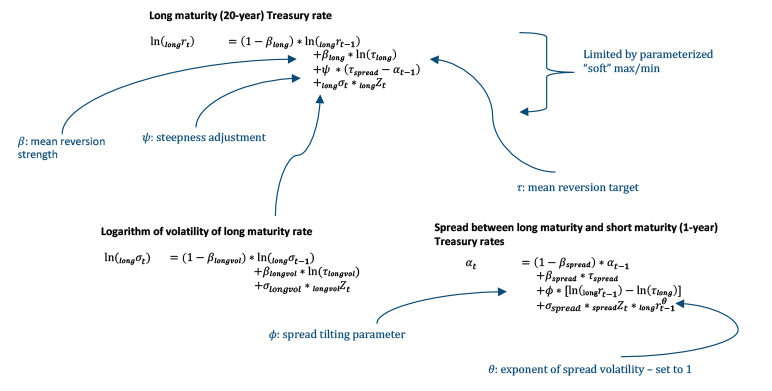
The model used by the AIRG, called the Stochastic Log Volatility (SLV) process, uses three related stochastic processes modeling the 20-year “long” Treasury rate, 1-year “short” Treasury rate, and a stochastic spread between the two. All three rates are derived under a similar mean-reverting process that pulls the rate toward a steady long-term average. The steady state average for the 20-year rate, called the mean reversion parameter (MRP), is a particularly important assumption and is the only parameter in the SLV process that is not set by the ESG.
A few notable features of the SLV interest rate model include:
- Steepness (ψ) and spread tilting parameters (𝜙) are applied to the long rate and spread processes, respectively, to reduce the likelihood of unrealistic inversion events compared to historical data.
- A fourth stochastic process was considered to model the stochastic log volatility of the spread process, but was deemed unnecessary.
- Short rates are floored at 0.4 percent and are set to be 25 percent of the long rate if the threshold is breached.
Bond and Equity Fund Returns
The bond and equity funds modeled by the AIRG are generated by separate processes. The bond process is straightforward, as shown in Figure 5.
Figure 5
Bond Fund Process
For each of the three bond funds, the mechanics (1) tie the fund return to the Treasury rate generated through the interest rate model at specific reference maturities, such as 10-years for the long duration corporate fund and (2) apply a spread adjustment appropriate for the riskiness of the underlying bonds. This enforces an internally consistent worldview between the interest rate process and the bond funds.
Figure 6
Equity Fund Process
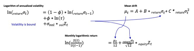
For equity funds, an alternative SLV process is used, similar to, but distinct from, the interest rate model. This model is one among numerous suitable options for equity fund projections and was found to sufficiently capture certain desirable equity return dynamics such as volatility clustering, negative skewness, and positive kurtosis.
A fairly straightforward mean-reverting process drives the log volatility, which serves as the volatility for the mean drift component. These components are then combined to produce the monthly log return.
Calibration
Having outlined processes and parameters, we will now cover calibration.
Interest Rates
The interest rate model is pre-parameterized and neither requires nor permits user intervention. The parameters are calibrated using maximum likelihood estimation over decades of collected history starting from the 1950s, with specific considerations including, but not limited to:
- The fit of long and short rates against historical averages.
- Reasonability of rates against historical extremes.
- Distribution of spreads against historical norms and inversion frequency.
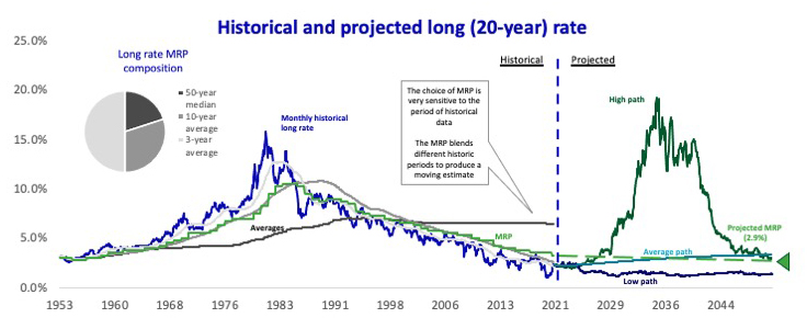
As noted previously, there is one particularly important parameter, the 20-year MRP, that is set by the ESG user using a prescribed blend (i.e., ratios and interpretation are prescribed and enforced by the ESG) of three-, 10-, and 50-year benchmark rates at the time of valuation; this allows the AIRG to be dynamic to evolving rate conditions without the need for constant rebalancing by the Academy.
Figure 7
Contribution of Historical Rates to the MRP
Bond and Equity Fund Returns
The fund return model is pre-parameterized and neither requires nor permits user intervention. According to the Academy, starting from 1950s monthly S&P data:
- Return percentiles fit history tightly.
- Show volatility clustering characteristics consistent with historical data.
- Large year-to-year drops appear with a consistent historical frequency.
- Kurtosis and skew characteristics align with historical norms, as shown in Figure 8.
Figure 8
Monthly S&P Returns
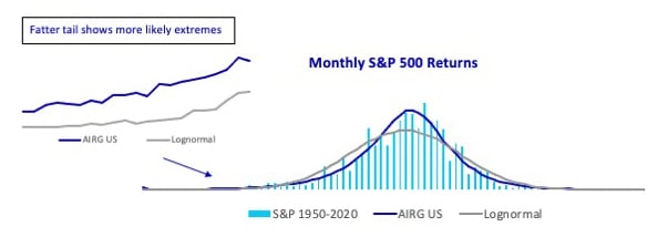
When comparing AIRG S&P 500 projections against a lognormal model parameterized to the same mean and volatility, the SLV has a tighter fit to the distribution of historic data. The AIRG exhibits some attractive qualities such as fatter tails and a skewed long left tail. Ultimately, the chosen parameters do rely on subjective judgement, such as evaluating historical interest rate patterns and defining a “reasonable” expectation of equity risk premium to set long-term return averages. The Academy periodically reviews the validity of underlying parameters.
Number
The number of scenarios within a scenario set is an important assumption as each scenario has a unique potential to expose different outcomes and risks. The AIRG can generate from 50 to 10,000 scenarios, but the user must decide on the appropriate number for the given use case. Using too few scenarios (e.g., 50) may not produce sufficient convergence. However, more scenarios (e.g., 10,000) may result in infeasible actuarial model runtimes.
Figure 9
CTE 98 for Sample GMAB Valuation
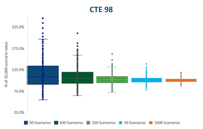
Consider the CTE figures for a sample GMAB valuation in Figure 9. When comparing against a 10,000-scenario benchmark, we see that the fewer scenarios we use, the less reliable our valuation, especially given the focus on extreme tail scenarios. Said differently, a 100-scenario result will only use two scenarios to inform CTE 98 valuation.
For US capital and reserving, using less than 10,000 scenarios requires the actuary to demonstrate that the subset will still pass prescribed calibration requirements, which are set using the full 10,000 scenarios. The percentiles of the best and worst 2.5 percent, 5 percent, and 10 percent of scenarios have to be “at least as extreme” as the calibration set.
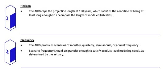
Time
Considerations around time, from the time horizon of scenarios to the frequency of generated scenarios is shown in Figure 10.
Figure 10
AIRG Time Considerations
Conclusion
The final and most important question is whether the outputs from the AIRG are appropriate for a given use case.
Given that the AIRG is prescribed for use in many reserving and capital contexts, it is by default the “correct choice” in those situations. More broadly, the ease of deployment and integration with many actuarial software platforms allows the AIRG to serve as a convenient “default option”; however, given certain limitations, biases, and inflexibility inherent in the AIRG, it is not necessarily an appropriate ESG for general-purpose real-world scenario generation.
The seven-step ESG decision-making process applied to the AIRG in this article provides a good case study on how actuaries can analyze a given ESG to understand and challenge the scenario sets upon which they so often rely.
The views or opinions expressed in this article are those of the authors and do not necessarily reflect the official policy or position of Oliver Wyman, the Society of Actuaries, or the newsletter editors.
Rahat Jain, FSA, CERA, MAAA, is a consultant at the actuarial practice of Oliver Wyman. He can be reached at Rahat.Jain@OliverWyman.com.
Dean Kerr, FSA, MAAA, ACIA, is a partner at the actuarial practice of Oliver Wyman. He can be reached at Dean.Kerr@OliverWyman.com.
Matthew Zhang, FSA, CERA, MAAA, is a senior consultant at the actuarial practice of Oliver Wyman. He can be reached at Matthew.Zhang@OliverWyman.com.