
Actuarial Problem Variety for Syllabi, Pedagogy, and Remediation
By Russell Jay Hendel
Expanding Horizons, November 2021

This article is written for instructors of courses covering material on the Society of Actuaries (SOA) and Casualty Actuarial Society (CAS) actuarial examinations. Instructors need a solid core of problems supplementing the learning objectives stated in their course syllabi. These problems point to noncontent skills that candidates must master for successful course mastery.
This article identifies three fundamental problem types and addresses how the (1) syllabus, (2) pedagogy and (3) remediation should present these problem types. The suggested approach increases candidate satisfaction and exam passing rates.
While the illustrative examples presented in this article are exclusively from the Financial Mathematics (FM) preliminary examination, the concepts identified apply equally to other preliminary examinations as well as the Fellowship examinations.
Relevant Concepts and Resources
Problem difficulty, a fundamental concept for examinations, is defined as follows:
Any individual question on an examination taken by several thousand students can be scored individually by calculating the percentage of candidates correctly answering the question. We call this percentage the problem difficulty. (An alternate approach bases difficulty on averages of subjectively reported numerical estimates of difficulty by knowledgeable experts).
Several software vendors providing actuarial problems publish problem difficulty. However, difficulty for problems on the preliminary examinations are not published. Instructors can also score difficulty on their own examinations.
One consequence of problem difficulty is that if the difficulty is too easy (e.g., 90%+) or too hard (e.g., 10%–), then that problem is not useful for future examinations because it will not adequately differentiate candidates. An ideal problem difficulty is about 50 percent, give or take 10–20 percent.
Any collection of problems affords an instructor, with access to its problems’ difficulties, the opportunity to seek common attributes in problems of similar difficulty; this article reports this author’s attempts. The article also shows how awareness of problem difficulty gives rise to different treatments in the syllabus, pedagogy and remediation. Other instructors are encouraged to make similar studies themselves.
Problems in this paper come from the Exam FM Sample Questions and Solutions (with one problem from the May 2005 FM examinations), publicly available on the SOA website. Readers are assumed to be familiar with the material in the FM course. A notation such as SQ#176 refers to Question #176 in the Sample Questions.
Two-Step Problems
The first problem type studied is called “two-step problems,” which are plug-in problems that create challenge by having multiple parts.
Example 1
SQ#176: An investor buys a perpetuity-immediate providing annual payments of 1, with an annual effective interest rate of i and Macaulay duration of 17.6 years.
Calculate the Macaulay duration in years using an annual effective interest rate of 2i instead of i.
Table 1
Model Solution to SQ#176
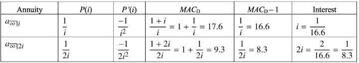
This solution is read from left to right in the second row and then from right to left in the third row: columns P(i), P′(i), MACD, and so on, give the perpetuity price, its derivative, its Macaulay duration, and so on, respectively. A crucial step in the multi-part solution is going from the calculated interest, i, in the last column of the second row to the 2i in the last column of the third row. Then, by reversing steps in the third row, we can calculate the requested problem value of 9.3.
This problem creates challenge by requiring repeated use of the MACD and perpetuity formulas; hence its classification as a two-step problem. The idea that doing a simple task twice is challenging is consistent with the idea of executive function, the capacity of the brain to deal with multi-task problems. Psychologists routinely use assessments presenting two-step problems to evaluate brain function.[1]
SQ#74 also presents a two-step problem whose solution can be modeled with a table similar to Table 1.
Example 2
Just as a two-step problem can be multi-part in the formula application, it can also be multi-part in the multiple parameters of a single formula.
SQ#178. A 20-year bond priced to have an annual effective yield of 10% has a Macaulay duration of 11. Immediately after the bond is priced, the market yield rate increases by 0.25%. The bond’s approximate percentage price change, using a first-order Macaulay approximation, is X. Calculate X.
The solution involves plugging into the formula,
![]()
This problem has two-step difficulty because although there is one formula, there are up to six variables (including expressions), i, i′, Δi, MACD, P(i′), and P(i). The problem gives three of these six variables and asks the candidate to calculate the ratio of two of the remaining three.
Two-Step Curriculum, Pedagogy and Remediation
It immediately follows that:
- The course syllabus, besides listing content objectives, should also list organizational objectives; for example, “You are expected to be able to solve multi-part problems.”
- Classroom instruction should emphasize both content (formulas) and organization of solutions.
- Remediation (student help) should also focus both on formulas and on organization. For example, a student who knows the formula should not be told, “You need more practice,” or “You need to learn your formulas better.” Rather it should be explained that “Besides knowing formulas, you should learn how to organize formulas into multi-part solutions.”
Monkey-Wrench Problems
A monkey-wrench problem, besides being two-step, has a “monkey-wrench,” something that can’t be done by a standard formula, typically an unexpected modeling.
Example 3
FM May 2005 Q21: A discount electronics store advertises the following financing arrangement: “We don’t offer you confusing interest rates. We’ll just divide your total cost by 10 and you can pay us that amount each month for a year.” The first payment is due on the date of sale and the remaining eleven payments at monthly intervals thereafter.
Calculate the effective annual interest rate the store’s customers are paying on their loans.
Monkey-wrench problems typically have a straightforward part, a solution component that is a routine plug-in. Letting C represent total cost, the timeline and equation of (present) value (PV; EOV) are straightforward. Figure 1 shows the time line for this example; the EOC is

Figure 1
Time Line for Example 3
![]()
A student may get stuck at this point since the solution requires, not another formula, but rather the identification of a hidden timeline, a nonexplicitly mentioned alternative method of payment—payment up front—required if the purchaser rejects the discount. The timeline for this second method of payment is a single cash flow of C at t = 0. Upon identifying the monkey-wrench, the problem reduces to a routine two-step problem where two methods of payment have identical PVs.
Example 4
A favorite among problem writers, whether of exams or textbooks, is to make problems multi-part since the problem then becomes a two-step problem. However, unlike Examples 1 and 2, which explicitly identified the two problems to be solved, in a monkey-wrench problem, there is an additional requirement to identify where and how to break up the problem into subproblems.
SQ#99: Jack inherited a perpetuity-due, with annual payments of 15,000. He immediately exchanged the perpetuity for a 25-year annuity-due having the same present value. The annuity-due has annual payments of X.
All the present values are based on an annual effective interest rate of 10% for the first 10 years and 8% thereafter.
Calculate X.
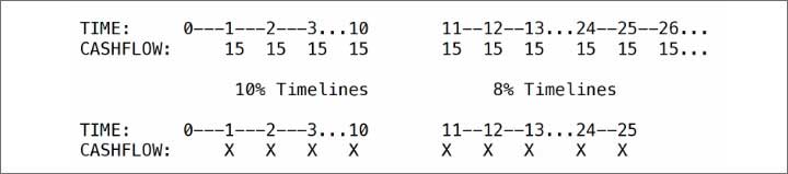
The solution requires identification of the two subproblems, with timelines from 0 to 10 and 10 to infinity respectively. This identification is the monkey-wrench. The application of formulas to each identified subproblem is then straightforward. Figure 2 presents the appropriate timeline breakups.
Figure 2
Four Time Lines at Different Interest Rates Used in the Solution of SQ#99
Research Problems
Research problem types are characterized by requiring trial and error to ascertain the correct method of solution. Research problems do occur on actual exams; knowledge of how to solve them is needed to pass. Learning objectives and remediation should emphasize a variety of research strategies such as divide and conquer, fail-first and solve-second, or generalization by analogy.
Example 5
SQ#114: Jeff has 8000 and would like to purchase a 10,000 bond. In doing so, Jeff takes out a 10-year loan of 2000 from a bank and will make interest-only payments at the end of each month at a nominal rate of 8.0% convertible monthly. He immediately pays 10,000 for a 10-year bond with a par value of 10,000 and 9.0% coupons paid monthly. Calculate the annual effective yield rate that Jeff will realize on his 8000 over the 10-year period.
The distinct feel of this problem, in contrast to those previously presented, should be clear. This problem is more than a two-step problem and more than a monkey-wrench problem. It is overflowing with subparts, challenging the candidate to know where to begin. Consequently, the candidate must experiment with different approaches, contrary to the plug-in culture candidates live in.
One approach that works for SQ#114 is divide and conquer: first solve recognizable problem components, and then integrate into a final solution. Figures 3 and 4 present the associated timelines for the loan and bond subproblems, respectively, bonds and loans being component units recognizable by the candidate. In each case, writing and solving the EOV is routine.
Figure 3
Time Line for Cash Flows for the Loan in SQ#114

Figure 4
Time Line for Cash Flows for the Bond in SQ #114

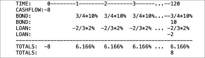
The last step in the solution, integration of the problem components, can be elegantly accomplished with a summary timeline, presented in Figure 5, which summarizes the net cash flow for each point in time. An EOV for the total line allows solving for i.
Figure 5
A Summary Timeline Integrating the Components of SQ#114
Example 6
The strategy for the following research problem is experimentation.
SQ#9. A 20-year loan of 1000 is repaid with payments at the end of each year. Each of the first ten payments equals 150% of the amount of interest due. Each of the last ten payments is X. The lender charges interest at an annual effective rate of 10%. Calculate X.
Where does one begin? One could note that if the outstanding loan balance at time 10, OLB10, were known, then an EOV could be set up relating OLB10 to the remaining 10 level payments of X. In attempting to find OLB10, it is natural to experiment with an amortization table as shown in Table 2.
Table 2
First Three Rows of an Amortization Table for the Loan in SQ#9
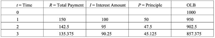
However, no pattern emerges. This type of initial failure experience is important in problem-solving but typically unknown to candidates. Additionally, failure should suggest trying an alternate approach, in this case algebraic, not numerical, as presented in Table 3.
Table 3
First Three Rows of an Amortization Table in Algebraic Form for the Loan in SQ#9
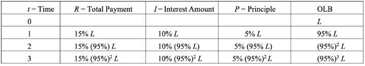
The pattern is now clearly visible, the implication that OLB10 = (95%)10 L is straightforward, and the solution to the problem based on a loan of OLB10 for 10 payments of X is then routine.
Example 7
The strategy for the following research problem is the use of analogy and generalization to create a new formula.
SQ #100: An investor owns a bond that is redeemable for 300 in seven years. The investor has just received a coupon of 22.50 and each subsequent semiannual coupon will be X more than the preceding coupon. The present value of this bond immediately after the payment of the coupon is 1050.50 assuming an annual nominal yield rate of 6% convertible semiannually. Calculate X.
The process of generalization by analogy is seen in the following three attempts:
- Attempt 1: The basic formula: Price = Coupon *
 + Cvn
+ Cvn
This formula does not help since the coupons are not level. - Attempt 2: Generalizing the formula: Price = PV of coupons + PV of C
This generalization provides a high-level verbal description of the algebraic formula in Attempt 1. - Attempt 3: Solve the problem by using an increasing annuity formula for the PV of coupons.
Conclusion
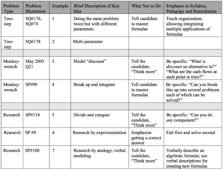
Besides advocating certain techniques, this article has advocated an attitude and perspective: Problems come in multiple types; each problem type has unique curricula, teaching, and remediation requirements. We believe such an attitude and perspective will assist instructors in improving their pedagogy. Table 4 summarizes our findings.
Table 4
A Summary of Classifications, Strategies and Examples Presented in This Article
Statements of fact and opinions expressed herein are those of the individual authors and are not necessarily those of the Society of Actuaries, the editors, or the respective authors’ employers.
Russell Jay Hendel, PhD, ASA, is adjunct faculty III at Towson University, where he assists with the Actuarial Science and Research Methods program. He can be reached at RHendel@towson.edu.