
Potential Modeling Challenges in a Negative Interest Rate Environment
By Zohair A. Motiwalla
The Financial Reporter, April 2022

This article shines a spotlight on some of the modeling challenges that practicing actuaries may experience when incorporating negative interest rates into their models. This recognizes that, even if interest rates are not currently negative, future rate expectations can be. The modeling challenges discussed here should by no means be construed as an exhaustive list. It is almost certain that different companies will have unique situations that may require special modeling treatment. This article serves to highlight awareness of negative rates and to prompt actuaries to ponder how the many models they use might need to be modified to appropriately accommodate such behavior.
This exercise is motivated in no small part by the proposed revisions to the National Association of Insurance Commissioners (NAIC) economic scenario generator (ESG). The new ESG is currently under development and the NAIC may require it to be used for principle-based statutory reserving (PBR) in the United States in the next few years. One of the key anticipated improvements in the new ESG relative to the existing version currently in use will be the ability to model negative interest rates, including “low for long” scenarios that can adversely impact profitability.
For a more detailed treatment of this topic, please refer to the report available online.[1]
Liability Considerations
On the liability side of the balance sheet, interest rates are often used to discount cash flows, as well as in annuity factor and dynamic lapse calculations.
The models used by actuaries may incorporate floors of zero percent on the interest rates that are used to derive discount factors when calculating the present value of cash flows. Alternatively, but equivalently, rather than a floor of zero percent on the interest rate, perhaps a cap of 100 percent on the discount factor is applied. Such code would need to be modified to accommodate negative interest rates and therefore discount factors greater than one. For risk-neutral modeling, failing to do so would potentially invalidate the results, as any flooring of the discount rates may result in a failure of the martingale test.
For spread business such as fixed deferred annuities or universal life, most models employ a dynamic lapse adjustment that is a function of the difference between an assumed market rate and the company credited rate on the policy. The market rate is a proxy for the credited rate used by a competitor company and is usually a function of the Treasury curve. The dynamic lapse adjustment for these spread products is commonly an additive adjustment to the company’s base lapse. The dynamic lapse function itself is commonly one-sided, meaning that an excess lapse (or positive additive adjustment to the base lapse assumption) is applied when the market rate exceeds the credited rate but when the reverse is true there is no lapse adjustment, i.e., the base lapse rate is not reduced. Thus, for a one-sided function an effective floor of zero percent is applied to the excess lapse whenever the market rate is less than the credited rate (which includes when the market rate is negative). For a two-sided function, care must be taken to ensure that the additive adjustment is sufficiently small so that the final lapse rate is not negative.
As a modeling convenience, actuaries will sometimes capture the lump sum present value of systematic lifetime withdrawal payments for a guaranteed lifetime withdrawal benefit (GLWB) on account value depletion rather than modeling the stream of payments over time. This lump sum present value will leverage an annuity factor calculation. For example, let’s suppose that under the company’s prudent estimate utilization assumption for PBR, a female GLWB policyholder chooses to elect her lifetime payments at age 45 and that, in the projection, the account value is fully depleted at attained age 60. Once this occurs, the remaining lifetime payments need to be funded out of the insurance company’s general account portfolio. If the actuary decides to calculate a lump sum present value of these remaining payments the model will calculate the annual life annuity factor for a female life aged 60 and multiply this by the contractual maximum annual withdrawal amount that this policyholder locked in at election at age 45. The interest rate used for the annuity factor is commonly based on the prevailing interest rates at the time the account value is depleted for the modeled economic scenario. A graph of the resulting annual life annuity-due factor for a 60-year-old female policyholder as a function of positive and negative interest rates is shown in Figure 1.
Figure 1
Annual Life Annuity-due Factor for a 60-year-old Female Policyholder as a Function of Interest Rates
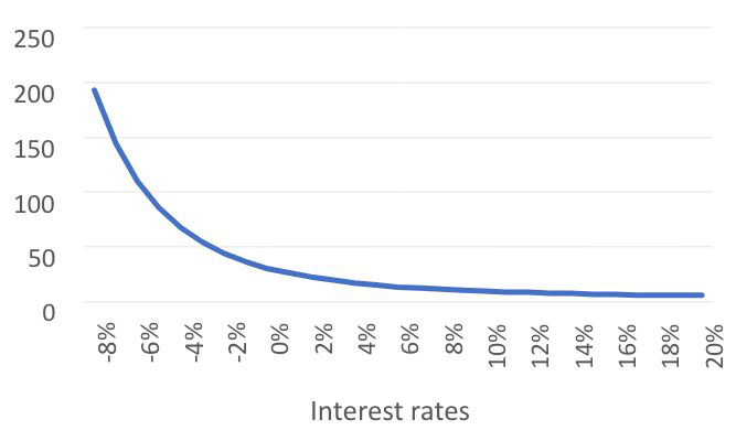
Note: Mortality is set to 80% of the 2012 Individual Annuitant Mortality Basic Table
We observe that the annuity factor is a monotonically decreasing function of interest rates. For positive and higher interest rates, the annuity factor decreases very slowly as the discount rate increases. However, for increasingly negative interest rates the annuity factor increases very quickly. For instance, with a 2 percent interest rate assumption, the annuity factor is 22.32, while for a -4 percent interest rate assumption, the annuity factor is 67.34. The current iteration of draft economic scenarios produced by the new NAIC ESG that is under development for PBR produces (unfloored) negative interest rates that fall to -8 percent. In our example above, a -8 percent interest rate assumption results in an annuity factor of 193.24, which is almost nine times as large as the annuity factor with a 2 percent interest rate assumption. On the surface, this certainly seems to strain our expectations for what constitutes a “reasonable” factor, but perhaps our expectations need to adapt to a new environment?
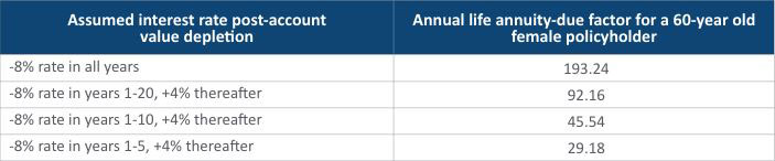
It is helpful to take a step back at this point and consider first principles. As actuaries our intuition has been informed by a lifetime of training to expect positive interest rates. However, mathematically there is nothing wrong with the annuity factors we are calculating in the example above. In this case, we can reconsider the interest rate approach that we are using for the discounting. The remaining liability that is created on account value depletion is essentially a single premium immediate annuity, with a duration that corresponds to the point on the Treasury curve that we can look at to determine an appropriate interest rate to use for discounting our annuity factor. When the rate is -8 percent, we know we get an annuity factor of 193.24. But what does using this -8 percent rate really mean? It means that we are locking in this rate from account value depletion and in every year thereafter. This is arguably a “low for long” scenario but taken to an extreme—is it reasonable to expect that the rate will always be -8 percent or can we expect a “recovery” to positive rates?[2] If one subscribes to the latter view, then instead of locking in a single rate we could instead use a series of rates for the discounting. For a given economic scenario, these rates would range from the prevailing rates at the time of account value depletion to those at the end of the projection.
Consider the illustrative table in Figure 2, which shows the annual life annuity-due factor for the same policyholder but using a varying interest rate assumption in the years after account value depletion. From this table, it is evident that a varying interest rate can have a significant impact on the annuity factor calculation, even with a prolonged negative rate environment. In practice, it would make more sense to discount each annuity cash flow by a relevant spot rate rather than using a single rate.
Figure 2
Annuity-due Factors Using Varying Interest Rate Assumption After Account Value Depletion
Asset Considerations
On the asset side of the balance sheet, the standard asset formulas used to discount cash flows when calculating the market value for fixed income instruments such as bonds should still work appropriately under negative interest rates. However, care should be taken to ensure that there are no floors of zero percent applied to the interest rates that are used to derive discount factors when calculating the present value of these asset cash flows, or that there are no caps of 100 percent on the discount factors.
Some actuarial systems may already be unintentionally producing irrational results in certain edge cases. For example, if a model utilizes borrowing to cover negative cash flows, a model might, in some cases, produce negative investment income on a negative asset balance and report a positive yield, which might then flow through into credited rate calculations. In scenarios where the asset balance is negative but close to zero, the reported yield might be hugely positive despite the company having no investment income available to cover the credited interest on the general account. Consider the following example:
- Bond book value = 100
- Bond yield = 4%
- Loan = 110
- Borrowing rate = 10%
The expected investment income is 4% * 100 – 10% * 110 = -7. And the invested asset balance is 100 – 110 = -10. Some systems might report this yield as 70 percent. Clearly the actuary would not want to use this 70 percent rate to drive credited rates. Reworking our example to use a bond yield of -4 percent and a borrowing rate of zero percent produces a similar outcome.
What earned rate should be used in cases such as these? One solution would be to floor investment income at zero when deriving the earned rate to be used for crediting. Because this produces an earned rate of zero percent, logic that floors the crediting rate at the guaranteed rate will then ensure that the latter “wins.” Of course, in a low or negative interest rate environment the company will experience liability spread compression because it must contractually credit the guaranteed rate despite earning insufficient expected investment income on the assets backing the liabilities.
Economic Scenario Considerations
The current iteration of draft economic scenarios produced by the new NAIC ESG produces negative interest rates that can go as low as -8 percent. There is some industry discussion of introducing a floor to prevent the real-world interest rates generated by the new NAIC ESG from falling below some threshold rate. At the time of writing this paper, this floor is still yet to be determined.
Concluding Thoughts
This article has briefly covered some of the modeling challenges that practicing actuaries may wish to consider when incorporating negative interest rates into their models. It is very likely that many other such challenges not discussed here also exist, and readers are encouraged to critically review the models that they use or are responsible for determining if and where negative interest rates might pose problems.
The timeliness of such actions is especially important considering the emergence of the new NAIC ESG that will produce negative interest rates, and the industry field testing for this generator that is expected to occur sometime during 2022. This industry field testing will provide an ideal opportunity for actuaries to determine the robustness of their models with respect to a negative rate environment and to grow their intuition of how negative interest rates can impact results.
Zohair A. Motiwalla, FSA, MAAA, is a principal & consulting actuary at Milliman. He can be reached at zohair.motiwalla@milliman.com.