
Interest Rate Interpolation—A Brief Excursion
By Maya Perelman and Bruce Rosner
The Financial Reporter, February 2022

Changes to financial reporting standards have generated renewed attention to discount rate curve construction. Interpolation between available data points is somewhat of a hidden issue buried in this process, with the potential for surprising depth. The majority of attention has gone toward extrapolation, focusing on what happens to the curve after the last liquid point. This is for good reason—it’s very impactful for certain long-duration products. This makes interpolation the less popular topic, with far less literature and exploration.
In this article, we leverage recent research and testing on this topic to provide actuaries with a basic education, and pointers on where certain methods may be more appropriate.
Overview of Interpolation Techniques
The first five interpolation methods shown below are adapted from Hagan and West’s paper, which can be referenced for further technical details on the algorithms[1]. We have also included the addition of Nelson-Siegel Svensson; further reading on this model can be found in Gilli, et al. 2010 paper[2].
- Linear interpolation on spot rates: Straight-line interpolation on the spot rates.
- Piecewise constant forward: With each segment of rates, the forward rate will be level. This method is also commonly known as raw interpolation, or linear on the log of discount factors.
- Piecewise continuous forward: This method builds off the previous one, and rather than restricting forwards to be constant for each segment, it allows them to be piecewise continuous linear functions.
- Splines: Polynomial interpolation of each segment in a way that each of the segments smoothly interconnects with the others. For example, a cubic spline typically constrains the level and the first and second derivatives at each knot.
- Monotone convex: An adaptation of Hyman’s monotone preserving cubic spline,[3] which adds a mechanism to ensure that the generated continuous forward rates are positive, given that the discrete forward rate inputs are positive. The key feature of Hyman’s spline is that it preserves the regions of monotonicity (i.e., successively increasing or decreasing) of the input values.
- Nelson-Siegel Svensson (NSS): A parametric curve fitted to model the term structure of the input rates. The model houses six parameters to capture the stylized features of a yield curve, such as long-run yield levels and time to maturity.
These six methods are not the full range of possible interpolation techniques; however, they do encompass some of the more popular techniques. Linear interpolation alone could be done a variety of ways, such as doing a log transformation before the linear interpolation. Additionally, we did not cover the Smith-Wilson method, which is more widely known as an extrapolation technique but is used for interpolation as well. Further reading on Smith-Wilson can be found in wide variety of sources, such as the CEIOPS’ Solvency II calibration paper[4].
Modeled Results
Exhibits 1 and 2 show results based on the US Single-A curve as of Dec. 31, 2020. Our process first assumes a conversion of the par yields to spot rates, and then performs the methods listed above to interpolate those spot rates. Some of the methods could have alternatively been applied directly to par yields.
Exhibits 1 and 2
Interpolated Spot and Forward Curves From US Single-A Input Yields as of 12/31/2020
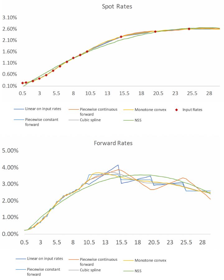
We immediately observe that the spot rates have limited room to deviate, while the forward rates show a larger spread. We also note that all of the spot curves pass through the input data points except for NSS, which applies a regression across the entire curve using a defined function.
We also compared the present value of a typical 30-year term life insurance policy discounted under each of the six initial curves shown above, and the present values ranged within 0.7 percent. On the other hand, for a bullet bond with a single cash flow at year 15, the NSS technique produced a result that was off by 2.2 percent from the other techniques. These indicative results show that in many applications, the final result may not be overly sensitive to the method chosen.
Below we consider key desirable features of an interpolation technique and assess which methods may fall short or particularly excel in that area.
Continuity of Forwards
Although each of the techniques produces continuous spot curves, we observe that linear on spot rates and piecewise constant forward rates have discontinuities at each segment endpoint. This makes these techniques less desirable from a theoretical perspective. To put it in simple terms, if the market actually traded sufficiently to produce a full curve, it is highly unlikely that it would result in these discontinuous shapes.
Monotone convex produces continuous rates along this curve; however, we note that we were able to generate discontinuities when feeding it certain unusual yield curve inputs, as displayed in Exhibit 4 seen in the following section. At the other end of the spectrum, NSS generates the smoothest curve as the lone parametric technique.
The practitioner should further consider the continuity of forward rates with regard to the connection with the extrapolation method being used. Possible techniques to ensure a smooth transition could involve constraining the first or even second derivative of the spot curve to zero at the last liquid point. If the second derivative can also be constrained to zero, then the forward curve will have a zero slope and grade nicely into a flat forward as well.
Stability and Locality
A key consideration is the stability of the rates with respect to small changes in the input rates. This also includes the concept of “locality”—that is, one would not expect a rate movement on the three-year tenor to have a large impact on the interpolated 22-year rate.
Cubic splines and piecewise continuous forwards are both notable violators of this locality principle. Exhibit 3 shows what happens to a cubic spline interpolation with a perturbation of 15 basis points up/down to the 10-year tenor. The slope in the yield curve at 10 years results in a dramatic rise and then fall. As the cubic spline algorithm attempts to match the first derivative at each segment, that pattern propagates throughout the curve. The piecewise continuous forward technique produces a similar response.
Some implementations of splines add additional constraints that help to mitigate this issue.
With Exhibit 4 we observe that monotone convex fares somewhat better; the oscillations affect fewer years but produce sharper discontinuities in the forward curve segments.
Exhibits 3 and 4
Forward Rate Curves Under the Cubic Spline and Monotone Convex Algorithms
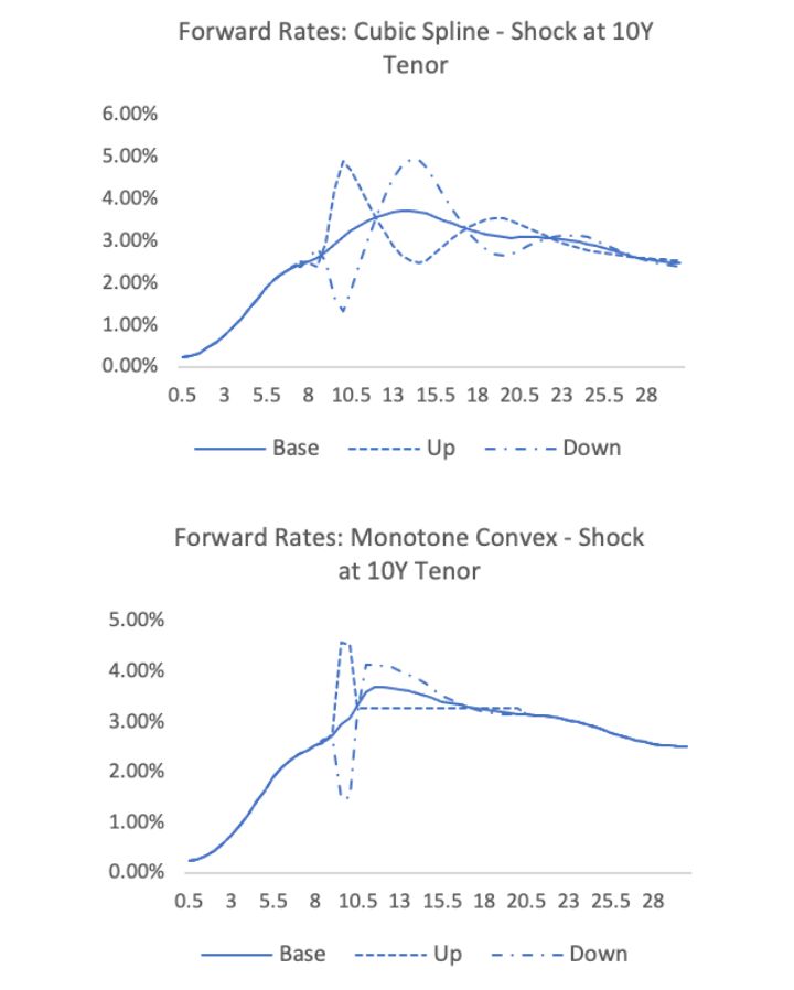
Note: The base curves are from the US Single-A curve as of Dec. 31, 2020. The up/down curves are based on shocks of 15 basis points applied to the 10-year tenor input.
The robustness of the NSS algorithm varies significantly depending on the given sensitivity applied to the input rate. For the above scenario of 15 basis point shocks applied to the 10-year tenor rate, the NSS algorithm remains relatively stable (Exhibit 5). However, applying a shock of the same magnitude but at the 20-year tenor instead, as depicted in Exhibit 6, can result in a dramatic shift of the entire parametric curve.
Exhibits 5 and 6
Forward Rate Curves Under the NSS Algorithm
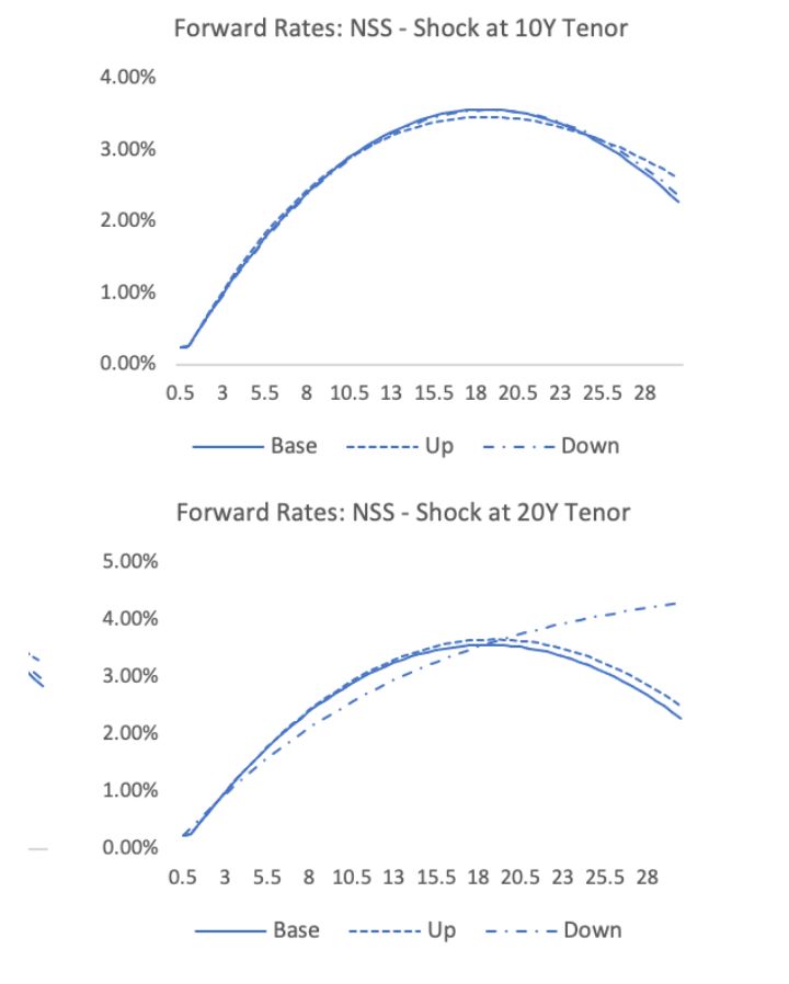
Note: Exhibit 5 depicts the curves given a 15 basis point shock to the 10-year tenor input, while Exhibit 6 shows the curves given the same shock applied but to the 20-year tenor.
Notably, linear interpolation and piecewise constant forwards are both perfectly local—a change to one segment has no impact on neighboring segments. We see a clear trade-off between stability and continuity, and one should weigh which of these is more relevant to the application.
Simplicity
Simplicity and ease of implementation are important characteristics of an interpolation method. Without a doubt, linear interpolation is at the forefront with respect to these features; it is widely used, well understood and straightforward to implement.
Piecewise constant forward rates simply involves linear interpolation on the log of the discount factors. And although this method may not be as broadly known, it is relatively easy to execute. Likewise, natural cubic spline interpolation is widely employed across the industry and therefore readily available, despite being more complex than some others discussed here.
The NSS algorithm can be fitted through common parametric approaches (e.g., least squares regression), however, numerical difficulties can be encountered in its calibration. Further, the NSS model is sensitive to the initial estimates of the parameters, and for certain ranges the model becomes unstable to small perturbations in the rates, as seen above. Considerations related to the NSS model calibration are further discussed in Gilli, et al., 2010 article.
The monotone convex and piecewise continuous forward algorithms are more complex than some of the others listed and may require significant up-front investment to implement.
Market Consistency
As already noted, NSS was the lone technique in this group that did not pass through the original input spot rates. This can be considered a feature or a flaw depending on the application. If the underlying data points are considered fully liquid, reliable market data, we probably don’t want to deviate from those. However, raw yield curves may contain varying degrees of liquidity, and can in fact occasionally have dislocations, such as a Single A rating showing a lower yield than a AA rating. A technique such as NSS makes more sense in a context where we are deliberately overriding the underlying data points with a shape that is somewhat predetermined.
Final Thoughts
Our analysis demonstrated that in many applications, the choice of interpolation technique will have only second-order impacts on financial results. In these cases, the decisions will likely be driven primarily by stability and simplicity. However, there are a variety of considerations, as well as the potential for sensitivity to different economic environments, and we expect that the industry will continue to apply a rich mix of practice, as we see today.
Statements of fact and opinions expressed herein are those of the individual authors and are not necessarily those of the Society of Actuaries, the newsletter editors, Ernst & Young LLP or other members of the global EY organization.
Maya Perelman, ASA, ACIA, is a consultant at Ernst & Young LLP (EY US) Consulting. She can be reached at maya.perelman@ey.com.
Bruce Rosner, FSA, MAAA, is a managing director at Ernst & Young LLP (EY US) Consulting. He can be reached at bruce.rosner@ey.com.