
Cluster Modeling: A Powerful Way to Reduce Cloud Costs
By Zohair A. Motiwalla and Aatman Dattani
The Financial Reporter, July 2023

The insurance industry is currently experiencing a period of disruption, with the ongoing legacy of the COVID-19 pandemic, rapidly rising interest rates and inflationary pressures, artificial intelligence, and data proliferation all having an impact on business-as-usual operations.
In the face of these challenges, it is more important than ever for actuaries to produce accurate and useful information in a timely fashion for all end-users and stakeholders. Seriatim actuarial models may be accurate, but they are often too costly and time-consuming to be useful for an effective and nimble response in a rapidly changing world. Accordingly, actuaries typically employ some form of proxy modeling in order to manage run-time.
A more recent reason for leveraging such techniques has been the gradual industry movement from a fixed cost on-premise grid to a scalable cloud solution for distributive processing. Moving to the cloud will reduce fixed costs and increase variable costs relative to an on-premise solution, with the increase in variable costs depending on a number of factors including the number of required sensitivities, “what-if” scenario management requests, and whether users are adhering to a model governance framework that determines when and how jobs are submitted to the cloud. Indeed, depending on the behavior of these users, the compute costs have the potential to dramatically accumulate, resulting in material and often unexpected financial outlays.
One proxy modeling technique that may help reduce these compute costs is cluster modeling, which allows users to submit “light” versions of their “heavy” production models to the cloud. A light model is in effect a version of the heavy model that runs substantially faster due to its being scaled down while still materially capturing the underlying economics of the heavy model. Cluster modeling draws on the well-developed theory of clustering in a statistical context. The technique intelligently maps similar “points”—potentially liability model points, economic scenarios, or asset CUSIP[1] numbers together in an automated fashion, allowing for a user-defined level of compression, while preserving the fit to within some reasonable level of tolerance to the heavy model. The “clusters,” which include various model points, are calibrated using financial metrics from the heavy model thus allowing for more accuracy in results and higher levels of compression than traditional techniques such as grouping.
Clustering and Key Performance Indicators Under U.S. Reporting Frameworks
A fair value reserve is calculated as the arithmetic mean result over a set of (risk-neutral) stochastic economic scenarios, effectively giving every scenario in this set an equal weight in the final result.[2] No prescribed regulatory floor is applied to this result. From a clustering perspective, the absence of a floor (or a cap) on this mean result implies a certain symmetry that, all else being equal, means there are fewer “artificial constraints” on the cluster calibration process. The same would hold true for a stochastic set of real-world scenarios over which a mean result is calculated—in other words, there is nothing particularly special about the use of risk-neutral scenarios in this context. Rather, it is the reporting metric or key performance indicator (KPI) and therefore the underlying framework specifying that metric that is key. Other proxy modeling techniques can also work well when considering the mean—for example, varying scenarios by liability model point, which for a sufficiently large in-force will generally require fewer scenarios to achieve convergence than a more conventional approach.
In contrast, the principle-based statutory reserves and capital framework in the United States uses a conditional tail expectation (CTE) result, defined as the mean over a small subset of the overall (real-world) stochastic economic scenarios. In a variable annuity (VA) context, a CTE 70 is calculated[3] for principle-based reserving (PBR) under VM-21 and a CTE 98 is calculated[4] for the total asset requirement under C-3 Phase II. The economic scenarios in question are generated each quarter using the currently prescribed American Academy of Actuaries Interest Rate Generator (AIRG). Under the statutory reporting framework for VAs, the heavy model effectively is a seriatim in-force file run over the full set of 10,000 economic scenarios[5] from the AIRG. Multiple variations of this heavy model may also need to be run in production.
Scenario and Liability Clustering
Most companies that sell VAs employ scenario, liability, and/or asset compression to produce a light model that is used for each of the variations described above. For scenarios, companies commonly use a subset of scenarios from the universe of 10,000 economic scenarios that are generated using the AIRG. The AIRG provides a scenario picking tool for this purpose, although it only leverages interest rates as a metric (or location variable[6]) to choose the scenarios. In contrast, clustering allows the use of any number of location parameters to choose scenarios thereby permitting companies to capture both equity and interest rate movements. (We refer to this approach as “Type I Scenario Clustering.”) An even more robust implementation of scenario clustering can be performed by first applying liability clustering and then using the light model output as calibration points for scenario clustering to develop a model that is lighter still.
In a statutory context, liability clustering for VAs involves running the heavy model over a small set of three to five economic scenarios (calibration scenarios) that represent the types of scenarios that would be modeled. Rather than focusing on the inputs, the output from the heavy model is captured over these calibration scenarios and used to develop the liability cluster. Importantly, this process ensures that the light model automatically captures the relevant policyholder behavior impact from the dynamic functions used to model such behavior in the heavy model.
More robust scenario clustering can then be performed by creating a (much more) heavily clustered liability in-force file, e.g., a 0.1 percent (1,000-to-1) cluster or even a 0.01 percent (10,000-to-1) cluster. Running a light model that uses such a heavily clustered liability in-force file would in all likelihood produce a less-than-desirable fit to the heavy model. However, the purpose of this heavily clustered in-force file is not to produce results for end-users, but rather to calibrate the scenario clustering more effectively. (We refer to this approach as “Type II Scenario Clustering.”) For example, companies could run the heavily clustered file over all 10,000 scenarios to produce output which, while somewhat inaccurate for reporting purposes per se, is much more informative to the scenario calibration process than an approach that simply focuses on the inputs since it captures the impact of the scenarios on the key business drivers.[7]
Practical Consideration and Limitations
Using clustering in this way can help increase the likelihood that the CTE metric that is produced with the light model matches to within a reasonable level of tolerance to what would have been obtained had the company run the heavy model (with all 10,000 scenarios).[8] That said, clustering, as with all proxy modeling techniques, often involves balancing what is most important to the actuary (and the company) with what might be considered less important. As an example, if statutory CTE 98 capital preservation is key, then the clustering can be calibrated so that the light model attempts to fit that KPI closely, while recognizing and accepting that by virtue of that increased focus there is the potential for slightly more noise in (say) the CTE 70 reserve. In general, matching to different KPIs is managed by calibrating the cluster to different scenarios and designing location parameters that capture the variability. There is a fine line between increasing the number of KPIs while simultaneously preserving a close fit on all these KPIs. Attempting to force the cluster to calibrate closely to many distinct KPIs will likely result in a worse fit overall.
In practice, it is also possible for asymmetries and/or nonlinearities in CTE results to occur. Examples of this might include when the cash value is binding in tail scenarios,[9] as it tends to be for out-of-the-money VA books, or where the Additional Standard Projection Amount is nonzero. These asymmetries can potentially distort any proxy modeling technique that is used, including clustering. Achieving a reasonable degree of fit is not an insurmountable difficulty in such cases, but often requires an experienced practitioner.
In certain circumstances, liability clustering may not be permitted by the reporting framework in question. For example, under the U.S. GAAP Long Duration Targeted Improvements, policies with market risk benefits need to be modeled on a seriatim basis. Using scenario reduction techniques (such as scenario clustering) in this context is a useful alternative that can reduce run-time.
Clustering can also be a powerful tool for performing attribution between reporting cycles as well as in pricing or business forecasting. Another important use case is running sensitivities for enterprise risk management purposes, where the actuary might be less concerned with whether the light model reasonably approximates the heavy model but rather that the light model sensitivity impact is close to the corresponding heavy model sensitivity impact.
Importantly, when liability clustering, we do not need to create different clustered liability in-force files for separate KPIs, but rather ensure that we calibrate the cluster to be robust enough across all such KPIs. Accomplishing this requires expert judgment in many cases and is where some art is needed.
Clustering Case Studies
Implementing Liability Clustering for a Variable Annuity Block
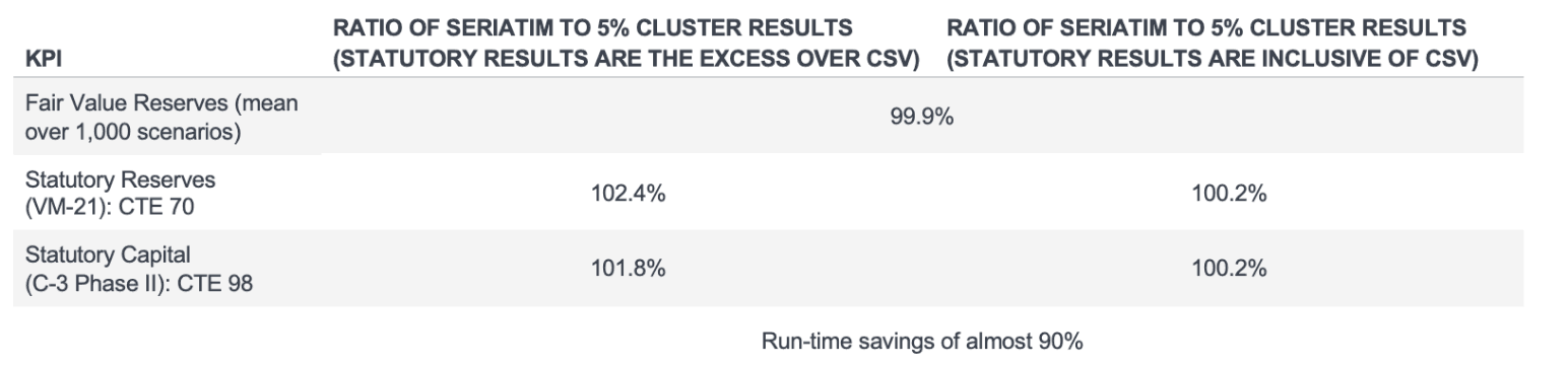
The VA block in this case study includes products with multiple riders—guaranteed minimum death benefits (GMDBs), accumulation benefits (GMABs), income benefits (GMIB), and lifetime withdrawal benefits (GLWBs). We implemented a 5% liability cluster on the block (a 20-to-1 or 95% reduction in liability in-force record count). The ratio of seriatim to 5% cluster liability results are shown in Figure 1, under statutory and fair value frameworks. For the statutory framework, we present CTE results both in excess of cash surrender value (CSV) and including the CSV. The seriatim run took half a day to run on the cloud and the 5% liability cluster run about 1.5 hours.
Figure 1
Ratio of Seriatim to 5% Cluster Liability Results
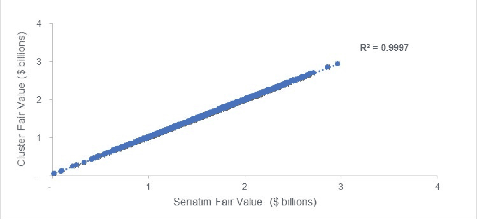
The graph in Figure 2 shows the fair value reserve using the seriatim (horizontal axis) versus cluster (vertical axis) compared across all 1,000 scenarios. The calculated R-squared measure for this data is almost exactly 100%.
Figure 2
Fair Value Result in Each of 1,000 Scenarios (In Billions)
We could have clustered the liability in-force file further, to say a 2% (50-to-1) or 1% (100-to-1) cluster model and achieved a similar fair value result fit. However, the desire to fit closely to the heavy model for multiple KPIs, namely the fair value, VM-21 reserve and C-3 Phase II capital, led to a decision to use a model with a more modest level of compression.
Conclusion
Clustering has the potential to help companies reduce run-time and therefore cloud computing costs in a wide variety of use cases. As with all proxy modeling techniques, understanding the purpose, business context, and downstream use of the light model is critical to calibrate the process properly and effectively.
For further details and additional case studies, we invite the reader to refer to the unabridged version of this article.
Statements of fact and opinions expressed herein are those of the individual authors and are not necessarily those of the Society of Actuaries, the newsletter editors, or the respective authors’ employers.
Zohair A Motiwalla, FSA, MAAA, is a principal & consulting actuary at Milliman. He can be reached at zohair.motiwalla@milliman.com.
Aatman Dattani, ASA, MAAA, is an associate actuary at Milliman. He can be reached at aatman.dattani@milliman.com.