
Alternative Experience Adjustment in LDTI DAC Amortization
By Steve Malerich and Janelle Kern
The Financial Reporter, July 2024

Since the American Institute of Certified Public Accountants (AICPA) added an alternative experience adjustment approach to its guidance on DAC amortization, we have encountered some misperceptions of what they mean by “the rate used to amortize DAC for the current reporting period” may be “calculated as of the beginning of the current reporting period using information known … at the end of the current reporting period … .”[1] This is often referred to as either the “alternative” or the “prospective” adjustment approach.
The misperception is that “information known … at the end of the current reporting period” means that amortization may be based on amounts in force at the end of each period. In this respect, the alternative method was meant to be the same as the FASB method, using amounts in force as of the beginning of each period. Hence, applying a higher amortization rate to an unchanged current basis produces higher amortization and no need for a separate experience adjustment for the reporting period.
In this article, we separate the AICPA’s illustration[2] into two steps: (A) Experience adjustment and then (B) assumption change. We then use the same illustration to demonstrate (scenario C) that applying the misperception would fail to produce the required experience adjustments.
Alternative Adjustment Deconstructed
The following illustrations begin after the example’s first year experience. In 20X1, $80 was capitalized, of which $16 was amortized. An additional $10 is capitalized at the beginning of 20X2 so that the total capitalized costs at this point are $74 (80-16+10). Note also that the AICPA illustration explicitly shows the basis in force as of the beginning of each year even when it uses information known at the end of a year.
Year 2—Experience Adjustment
Step A includes actual 20X2 experience but not the assumption change. Since the original calculations assumed no lapses, the actual 20X2 experience reduces the amount in force at the beginning of year three (“information known … at the end of” 20X2). With an unchanged zero-lapse assumption, that amount is projected to remain in force for the remaining term to expiry.

As in the AICPA’s Schedule Three, the total basis (x) sums the amounts in force as of the beginning of each year.
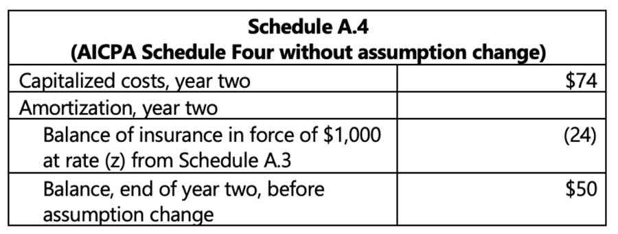
Applying the updated amortization rate to insurance in force at the beginning of 20X2 produces $24 of amortization, $5 more than the $19 illustrated in Accounting Standards Codification paragraph (ASC) 944-30-55-7B before the experience adjustment.
Year 2—Assumption Change
A 20X2 assumption change has no effect on actual amounts in force at the beginning and end of 20X2 (beginning of 20X3). Step B introduces a non-zero lapse assumption for the projection into subsequent periods.
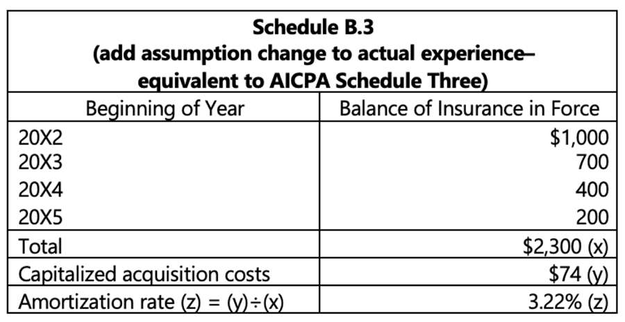
The total basis in Schedule B.3 sums the amounts in force as of the beginning of each year.
Having successfully reproduced the results of the AICPA alternative experience adjustment approach, we turn next to what happens if amortization is based on amounts in force at the end of each period.
End-of-Period Basis
Before we can demonstrate how the faulty experience adjustment fails to satisfy the requirement, we first need to recognize another concern introduced when amortization is based on end-of-period in force.
When amortization is based on end-of-period in force, DAC is fully amortized before the final period in a projection. In practice, this is unlikely to ever have a material effect on amortization. For example, fully amortizing over 159 quarters of a 40-year maximum life won’t materially distort DAC amortization even if we expect every contract to remain in force for the full 40 years.
In the simple example illustrated in ASU 2018-12 and in the AICPA guide, dropping one year from a five-year maximum term is significant and could distract us from the more important issue of experience adjustments. To avoid that distraction, we illustrate this as if contracts persisting to 20X5 remain in force at the end of 20X5 (and then terminate immediately after).
Year 2—Experience Adjustment
As in Step A, scenario C includes actual 20X2 experience but not the assumption change. The actual 20X2 experience reduces the amount in force at the end of year two. Since the original assumption is for zero lapses, that amount is projected to remain in force to the end of 20X5.
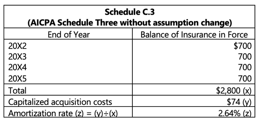
Unlike the AICPA’s Schedule Three, the total basis in Schedule C.3 sums the amounts in force as of the end of each year.
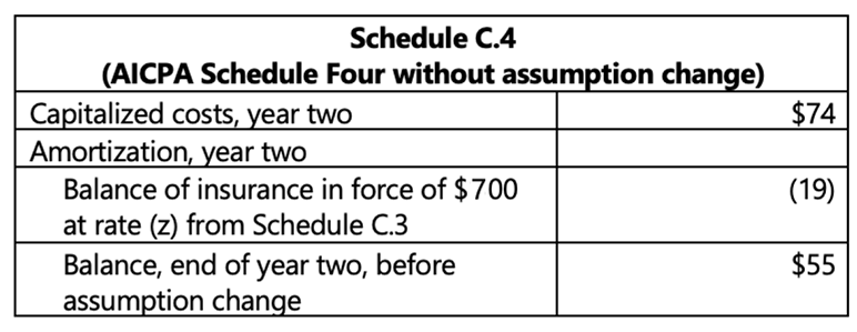
As shown here, applying the alternative adjustment method using end-of-period amounts in force does increase the amortization rate. But applying the higher rate to the reduced in force balance removes any experience adjustment. The $19 amortization in year two is the same amount shown in Schedule Four of ASC 944-30-55-7B—before the experience adjustment. In this case, the alternative approach failed to reduce the “balance of capitalized acquisition costs … for actual experience in excess of expected …” (ASC 944-30-35-3B).
To show that this is not a unique outcome of one particular example, we next demonstrate in formula that it is generally true.
Adjustment Formula
Amortization based on end of period amounts in force can be shown formulaically by an adaptation of the formulas presented on page 87 of the American Academy of Actuaries practice note, Application of ASU 2018-12 to the Accounting for Long-Duration Contracts under U.S. GAAP, December 2023.
When amortizing on end-of-period in force, the amount in force at the beginning of period t (Basic in Forcet-1) is dropped from the denominator of the amortization rate formula (kt). The formula for end of period DAC is similarly modified, applying the amortization rate to end of period in force.
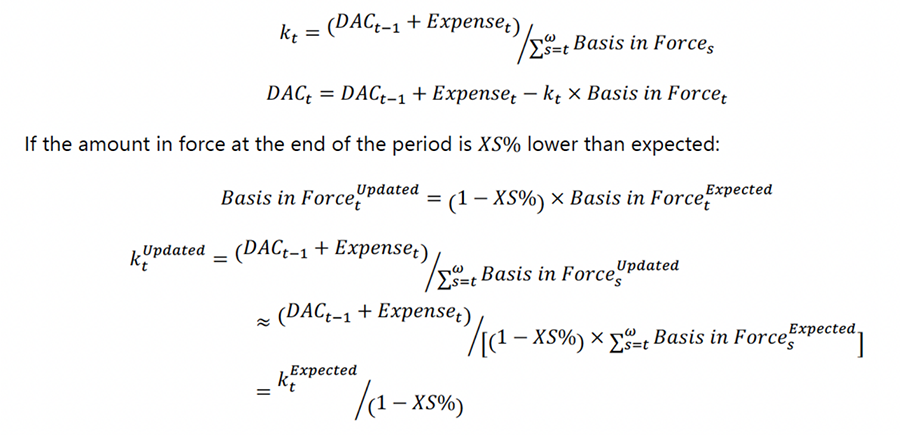
In a homogeneous cohort, the approximation in this formula would be an equality. In a real cohort, the total projected basis won’t vary by the same proportion as the aggregate deviation from expected in force. With individual contracts having different lengths of expected terms within the cohort, the updated amortization rate may be more or less than this approximation would produce.
Applying this updated amortization rate to actual in force at the end of the period:

In words—the alternative adjustment approach has approximately no effect when amortization is based on end of period in force.
Of greater concern—adjustments will be uncorrelated with the direction of variance! The direction of the adjustment depends not on the direction of variance but on characteristics of which contracts unexpectedly terminate or persist.
For example, suppose our illustrative cohort included some seven-year term contracts in addition to the illustrated five-year term contracts.
- Excess terminations among the seven-year contracts will reduce projected in force by more than the overall excess termination rate. DAC amortization will be greater than expected and the approach will appear to satisfy the ASC 944-30-35-3B requirement.
- In contrast, excess terminations among the five-year term contracts will reduce projected in force by less than the overall excess termination rate. DAC amortization will be less than expected—a clear violation of the requirement.
Interim In Force
Before closing, we recognize a variation that we have seen. In this variation, amortization is based on a sum or an average of amounts in force at the end of interim periods within a reporting period. For example, second quarter amortization is based on the average of amounts in force at the end of April, May and June.
In this case, the alternative approach will fail to adjust for actual experience during the first interim period but will adjust for experience during the remaining interim periods. This will sometimes lead to favorable experience adjustments even when actual experience is worse than expected.
Continuing the example, suppose April lapses are two percentage points higher than expected, May lapses are one percentage point lower than expected, and June lapses are as expected. In this case, total lapses are higher than expected during the quarter but the alternative approach using average end-of-month amounts in force would amortize less than expected.
Conclusion
GAAP does not explicitly state that amortization must be based on amounts in force as of the beginning of each period. However, when amortization is based on amounts in force at the end of each period, the alternative experience adjustment fails to satisfy the requirement in ASC 944-30-35-3B to reduce the balance for actual experience in excess of expected.
Statements of fact and opinions expressed herein are those of the individual authors and are not necessarily those of the Society of Actuaries, the newsletter editors, or the authors’ employer.
Steve Malerich, FSA, MAAA, is a director at PwC. He can be reached at steven.malerich@pwc.com.
Janelle Kern, FSA, MAAA, is a director at PwC. She can be reached at janelle.d.kern@pwc.com.
Endnotes
[1] American Institute of Certified Public Accounts, Audit and Accounting Guide - Life and Health Insurance Entities, Appendix A, paragraph A.72.