Defining a Posteriori Distribution of a Long-Term Rate Structure: A Mixed and Empirical Approach Based on Fisher’s Formula

By Octavio Rojas

International News, January 2023

This article is based on an analogous paper presented at the ASTIN-AFIR 2017 Colloquium held in Panama City, Panama. It sets an updated view of the problem, given the current thread of high inflation all over the world due to (among other events) the COVID-19 pandemic and the conflict between Russia and Ukraine.

A point to bear in mind is that, although the paper was within the framework of the International Accounting Standards, both the U.S. Financial Accounting Standards Board (FASB) and the International Accounting Standards Board (IASB) define a highly inflationary environment as that which has attained three-year accumulated inflation close to 100 percent. This is unlikely to occur in OECD countries but is already experienced in Venezuela and several other countries.

Countries that should be reporting under IAS 29 have similar requirements as those of FAS 52. The difference lies in the procedures to comply with their respective standards.

The above procedures are meant to apply to any country/environment where IAS 29 applies. Thus, it does not have to be considered hyperinflationary per the definition set by economists (a country that has two or more months in a row with a CPI greater than 50 percent).

The algorithm used:

1. Can be applied to any economic environment where:
• There exists a poorly performing stock market,
• Government Bonds are issued on an irregular basis or have been considered to be privately allocated,
• It complies with the definition of a high inflationary environment, and/or
• Information on long-term inflation does not exist or is too difficult to determine or forecast
2. Aims to define a real discount rate by deriving the embedded inflation rate assumptions from the average nominal rates on government bonds,

Further, the fact that the accounting statements do not provide explicit direction in these cases leads to multiple interpretations, including setting rates based on “rules of thumb,” making it difficult for proper peer review, or for a practicable International Standard of Actuarial Practice (ISAP) on this issue to be published.

For other financial assumptions (salary increases, pension increases, etc.), real rates can be defined in terms of current inflation. Nevertheless, if we were to use long-term nominal salary increases based on a calculated real salary increases, the corresponding real long-term inflation rates should apply.

We now formally present a procedure to define a real discount rate, by estimating long-term inflation, which attempts to deal with the loophole set in the referred accounting standards.

We should mention that the procedure has been developed to produce real rates, regardless of the economic environment or the ambiguity presented in paragraph 76 of IAS 19, given that it does not provide a way to measure when (and why) real rates should be considered as more reliable than nominal rates. Thus, many practitioners solely use real rates when IAS 29 applies because paragraph 76 indicates through an example that real rates should be used, but they do not describe how to identify other conditions where real rates should also be used.

We present a basis for opening a debate on this subject to help raise quality standards within the actuarial and accounting community.

In Venezuela: Are Government Bond Yields Linked with Inflation?

Our earlier paper proved that such conditions applied in Venezuela from 01/2003 to 12/2015.

So, our first task is to demonstrate that such a condition persists after 12/2015.

From 12/2015

The high costs of placing Government Treasury Bonds (GTB) in the market due to lack of buyer interest required their being sold at discount, making interest payments more expensive. The government then changed its strategy (much in line with other countries) and decided to first re-purchase their debt and afterward privately place it.

The above has led to the trend shown in Figure 1.

Figure 1
CPI vs Discount Rates

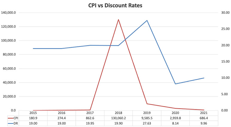
Source: Central Bank of Venezuela.

Within the period the Venezuelan currency suffered two major devaluations:

• During the third quarter of 2018, five zeros were taken off from the currency, giving place to a new denomination and a huge increase to the minimum salary. So much was the impact that during the period 11/2018 to 02/2019, Venezuela experienced an average monthly CPI of 132.4 percent.
• 12/2020 TO 01/2021: Six further zeros were eliminated from the currency. Given the way prices had increased before then, people were used to expressing prices in terms of millions so, its impact was not as great as that during 2018, subsequently slowing the perceived rate of inflation.

Based on the above, we can state that the Venezuelan Government Bond Yield (GBY) is still linked with inflation.

The Algorithm

Figure 2
The Algorithm
Defining the initial parameters:

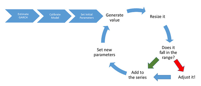
1. Define the best estimate for the CPI monthly series from a GARCH(p,q) model
1. Define the average nominal government (or corporate) bond rate as of date (R)
2. Define an initial confidence interval based on the results of the model and R
3. Modify/change the model so it can serve for the purpose of forecasting
2. Calculations per chain:
1. Define a confidence interval at time t based on the CPI’s history as of the previous month, which will have information from the historical data and the estimated results up to then
2. Generate an estimate from the modified GARCH(p,q) model:
1. If the estimated amount falls within the confidence interval, it will be added to the series
2. Otherwise, if:
• The estimated amount is less than the lower limit, the difference will be added to the lower limit
• The estimated amount is greater than the upper limit, the difference will be subtracted from the upper limit

In any case, the resulting amount shall be within the range of the interval, taking as the next value of the series.

A total of 5,000 iterations of length 420 future months were drawn, for a future time-span of 35 years.

Applying the Algorithm: Results

Following are the results of each phase of the algorithm, presented in the same order as in the previous section.

1     Defining the initial parameters

1.1     Define the best estimate for the CPI monthly series from a GARCH(p,q) model

By using parts of the code presented by Zivot (2012), we got our first set of results. These are

GARCH MODEL FIT
CONDITIONAL VARIANCE DYNAMICS
GARCH MODEL: sGARCH(1,0)
MEAN MODE: ARFIMA(0,0,0)
DISTRIBUTION: norm
OPTIMAL PARAMETERS:

	Estimate	Std. Error	t value	Pr(>|t|)
mu	0.044414	0.003455	12.8535	0.000000
omega	0.000122	0.000050	2.4103	0.015938
alpha1	0.999000	0.127721	7.8217	0.000000

1.2     Define the average nominal government (or corporate) bond rate as of date (R)

To be able to use Fisher’s formula, we need to derive the average nominal long-term discount rate. To do so, we make use of the information issued by the Central Bank of Venezuela as of 12/2021, in its “Tasas de Interés de Política Monetaria.” Table 1 provides only the rates of the privately placed GTBs. According to Table 1, the interest rate as of 12/2021 was 10.13 percent.

Table 1
INTEREST RATES OF MONETARY POLICY INSTRUMENTS

CENTRAL BANK OF VENEZUELA INTEREST RATES OF MONETARY POLICY INSTRUMENTS (PERCENTAGES)
Year / Month	Direct Allocation
2022	14.21
03	16.25
02	16.25
01	10.13
2021	9.96
12	10.13
11	10.13
10	10.13
09	10.13
08	10.13
07	10.13
06	10.13
05	10.13
04	10.13
03	10.13
02	10.13
01	8.13
2020	8.14
12	8.13
11	8.13
10	8.13
09	8.13
08	8.13
07	8.13
06	8.13
05	8.13
04	8.13
03	8.13
02	8.13
01	8.25
2019	27.63
12	8.13
11	8.00
10	34.15
09	34.16
08	34.01
07	34.00
06	34.00
05	34.00
04	31.09
03	30.50
02	30.50
01	19.00
2018	19.90
12	19.00
11	19.00
10	19.00
09	20.55
08	19.00
07	20.55
06	20.55
05	20.55
04	19.00
03	20.55
02	20.55
01	20.55
2017	19.95
12	20.55
11	19.00
10	21.07
09	19.00
08	19.00
07	20.55
06	19.00
05	19.00
04	20.55
03	20.55
02	20.55
01	20.55
2016	19.00

 

1.3    Define an initial confidence interval based on the results of the model and R

Based on an annual inflation rate equal to the interest rate of the previous step (10.13 percent), our initial 90 percent confidence interval is (-0.014209, 0.030356).

1.4    Modify the model so it can serve for forecasting purposes

To start, we should first focus on our task, which is for the long-term rate to comply with Fisher’s formula, which states that for a nominal long-term rate i

ln(1+R)=ln(1+r)+ln(1+i) (1)

So, if R equals 10.13%, then i ∈ (0.00%,10.13%).

Now, given that we are forecasting, our formula is written as follows:

ln(1+R)=ln(1+r_t )+ln(1+i_t) (2)

So that the condition should apply at any point t ∈ {0,1,2,…}

From Section 1.1, we have deduced that, unless we change the model:

• There will come a time when the values will all converge.
• All values will fall outside the boundaries of the model, given that the last known values will produce an annualized value greater that 10.13 percent

To avoid the above, the following steps were taken:

• In the original formula, for forecasting purposes we replaced with where is the average value of , from 0 to t, multiplied by the absolute value of v~N(0,1).

Thus, the above, gives place to the following:

(3)

Where: and 0 the starting point

• Finally, to comply with the condition that at every point in time, the value (1+h_t )¹² - 1 < 10.13%, the value of h_t will be multiplied by:

(4)

The reasons that the above number is so small in comparison to the one for 12/2015, is:

• The reduction in the target (10.13 percent vs. 16.00 percent)
• The increase of standard deviation in the CPI due to the devaluations that occurred during the period 12/2015 to 12/2021

2     Calculations per chain

2.1    Define a confidence interval at time t

After each iteration, we calculate a new average and standard deviation by adding to the series. Then we recalculate new upper and lower interval limits using the same procedure described in Section 1.3.

2.2    Generate an estimate from the modified GARCH(p,q) model

To generate each new value we;

• Recalculate  by using formula (3)
• Multiply the above result by Ψ
• Follow the procedure to define the value added to the series 

After a total of 5,000 iterations of length 420 (equivalent to 35 years), the results of the real rate conditioned to the embedded inflation within the 10.13% rate are shown in Figure 3.

Figure 3
Real Yield Curve

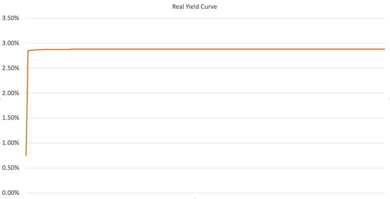
Figure 3 provides a trend which is very near to that of a flat yield curve. This curve indicates that short-term yields reach long-term yields at a very fast pace. This is a very promising result given that:

• It reflects the government’s position to rule over future interest payments by creating a sense that the country is at the beginning of a period of economic growth, and
• The necessary information to generate a proper yield curve is not explicitly available.       

It is of great importance to point out that unlike the yield curve obtained as of 12/2015, when the Venezuelan market had Government Bonds issued at different dates and with different terms and interest rates, giving rise to a normal yield curve, as of 12/2021 the yield curve is practically flat, something which is in line with the view expressed about the type of the Venezuelan yield curve in IAA’s book, Discount Rates in Financial Reporting. This implies that for a flat yield curve to exist, the market of Government Bonds has to be 100 percent privately allocated.

We can conclude that, from our point of view, the aim of the procedure was achieved and that the methodology used is consistent with both financial and economic principles. In the following section we shall further support our conclusion.

Goodness of the valuation results and next steps

To value the goodness (or reasonableness) of the results, we first calculated the average real rate of the model as of 12/2021. This resulted in an approximate value of 2.88 percent.

To see whether this result is reasonable (meaning that it falls within a range of countries that have a stable economy), we make use of the information provided by Willis Towers Watson in their “2022 Global Survey of Accounting Assumptions for Defined Benefit Plans.” Within its report, they present the following table:

According to Figure 1 of WTW’s “2022 Global Survey of Accounting Assumptions for Defined Benefit Plans,” our value as of 12/2021 (2.88 percent), falls between the average rates for IAS 19 purposes as of 12/2021 used in Canada (2.95 percent) and the United States (2.80 percent). Apart from this, Venezuela fully complies with IAS 29, paragraph 3, part b which states that "… the general population regards monetary amounts, not in terms of the local currency but in terms of a relatively stable foreign currency…” In the Venezuelan case, such foreign currency is the U.S. Dollar.

Based on the above, we can conclude that our goal of getting a rate that complies with the condition set in paragraph 76 of IAS 19 has been achieved.

Final Remarks

Although this article can be considered to deal with hyperinflation, the algorithm used can relate to non-hyperinflationary environments by changing the type of model used (GARCH) with a model more suited to high but non-hyperinflationary economies.

Statements of fact and opinions and calculations expressed herein are those of the individual authors and are not necessarily those of the Society of Actuaries, the editors, or the respective authors’ employers.

---

Octavio Rojas is an accredited actuary in Caracas, Venezuela. He has a BSc in actuarial science from Universidad Central de Venezuela and studied stochastic methods in Edinburgh, Scotland. Currently, he represents the Caribbean Actuarial Association (CAA) in IAA’s Pension Accounting Committee.