
Deep Learning for Liability-Driven Investment
By Kailan Shang
Risks & Rewards, February 2022

This article summarizes key points from the recently published research paper “Deep Learning for Liability-Driven Investment,” which was sponsored by the Committee on Finance Research of the Society of Actuaries. The paper applies reinforcement learning and deep learning techniques to liability-driven investment (LDI). The full paper is available at https://www.soa.org/globalassets/assets/files/resources/research-report/2021/liability-driven-investment.pdf.
LDI is a key investment approach adopted by insurance companies and defined benefit (DB) pension funds. However, the complex structure of the liability portfolio and the volatile nature of capital markets make strategic asset allocation very challenging. On one hand, the optimization of a dynamic asset allocation strategy is difficult to achieve with dynamic programming, whose assumption as to liability evolution is often too simplified. On the other hand, using a grid-searching approach to find the best asset allocation or path to such an allocation is too computationally intensive, even if one restricts the choices to just a few asset classes.
Artificial intelligence is a promising approach for addressing these challenges. Using deep learning models and reinforcement learning (RL) to construct a framework for learning the optimal dynamic strategic asset allocation plan for LDI, one can design a stochastic experimental framework of the economic system as shown in Figure 1. In this framework, the program can identify appropriate strategy candidates by testing varying asset allocation strategies over time.
Figure 1
LDI Experiment Design
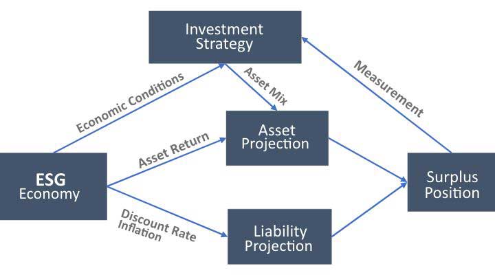
Deep learning models are trained to approximate the long-term impact of asset allocation on surplus position. RL is used to learn the best strategy based on a specified reward function. It is a forward, semi-supervised learning algorithm. This means that only the current impact is observable until the end of the experiment. However, with enough experiments, RL is expected to learn the characteristics of successful strategies and identify the ones that maximize reward. These dynamic investment strategies will then choose the action that maximizes the reward at each decision point in each scenario. However, these strategies may not be optimal ones because RL does not evaluate the entire space of possible asset allocation paths.
Figure 2
RL Process for LDI Strategy
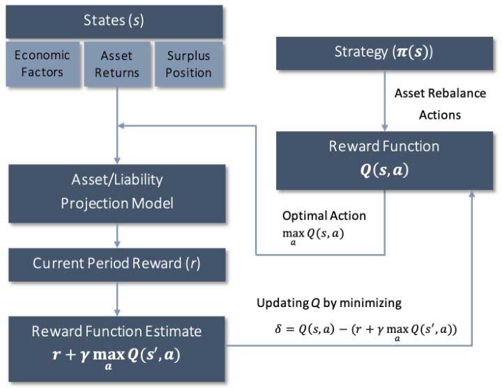
Figure 2 shows the RL process used to derive the investment strategies. The goal is to find the optimal dynamic investment strategy π*(s) based on s, the states that decision makers can observe at the time of decision-making. The states are economic conditions and surplus position. The optimality of an investment strategy is defined as the one that maximizes the reward function Q*(s,a) determined by s, the states, and a, the rebalancing action determined by the strategy π*(s):
![]()
The reward function Q*(s,a) is difficult to define. The impact of an asset mix selection not only affects current period performance but could also have long-lasting impact on the future surplus position. And impacts on future periods are difficult to estimate given the uncertainty of future economic conditions and surplus positions. For example, an inappropriate asset mix may cause a sufficiently deep deficit that is unlikely to be recovered based solely on future higher asset returns. Starting from a large deficit position, even when the asset return exceeds the liability return, the deficit could still increase because the starting liability value is larger than the asset value. Instead of defining the reward function directly, it can be constructed in a recursive form:
![]()
where
r: current period reward that can be observed; for example, it could be defined as the change in either the surplus amount or the funding ratio,
γ: discount factor to reflect the timing difference, and
Qπ(s',π(s')): reward function in the next period with new states s' and new asset rebalance action π(s')
Q(s,a) is a reward function that explains nonlinear relationships. Q is the sum of the current period reward and discounted rewards in the future, assuming that future optimal actions will be taken based on Q. It is structured as the Bellman equation used in dynamic programming to describe value given state and action, except that unlike dynamic programming, the exact function in RL is not defined but rather learned by minimizing the error δ between the two sides of the recursive equation:
![]()
RL is a forward process where only the current reward can be observed, and all future rewards can only be estimated based on just the existing Q. However, traditional model training needs the true value of Q, which is unknown. To address this calibration challenge, RL tries to match the current reward r and the change in Q, measured as ![]() . By doing that, the observed current reward can be used to keep improving the accuracy of Q. Using deep learning models such as feed-forward neural networks and long short-term memory models, the actual reward function can be approximated without needing to set the exact functional form before model training. With enough experiments, theory states that the calibrated Q function will be good enough to advise a good, if not optimal, action.
. By doing that, the observed current reward can be used to keep improving the accuracy of Q. Using deep learning models such as feed-forward neural networks and long short-term memory models, the actual reward function can be approximated without needing to set the exact functional form before model training. With enough experiments, theory states that the calibrated Q function will be good enough to advise a good, if not optimal, action.
As shown in Figure 2, the experimental environment is used to generate different states so the model can test different investment strategies and find the optimal one. The asset rebalance action that has the highest expected reward is chosen and modeled to calculate its impact on current period performance. As additional scenarios are tested, the deep learning model representing the reward function is updated and expected to move closer to the real reward function.
The RL process described above is also known as deep Q-learning, in which deep learning models are used to represent the reward function and the Q value is learned and optimized with respect to action a.
To evaluate the effectiveness of RL compared to traditional strategic asset allocation methods, a sample DB plan was modeled with economic scenario generation, dynamic liability projection, asset allocation and surplus projection. The comparison between optimal static investment strategies and RL-based dynamic strategies was performed assuming two asset classes: An AA-rated corporate bond portfolio and large-cap public equity. Efficient frontiers are built assuming fixed time horizons and static investment strategies, as shown in Figure 3. Blue dots stand for efficient frontiers at different time horizons based on static investment (i.e., constant asset mix) strategies. Both fully connected neural networks (FCNN) and long short-term memory (LSTM) models were used to approximate the reward function in the RL process, shown as triangles and black squares, respectively. The resulting dynamic investment strategies show that RL is able to generate reasonable investment strategies with the potential for generating better risk-return tradeoffs than optimal static strategies that have a target time horizon.
Figure 3
Dynamic Asset Allocation: Two Asset Classes Without Rebalance Constraint
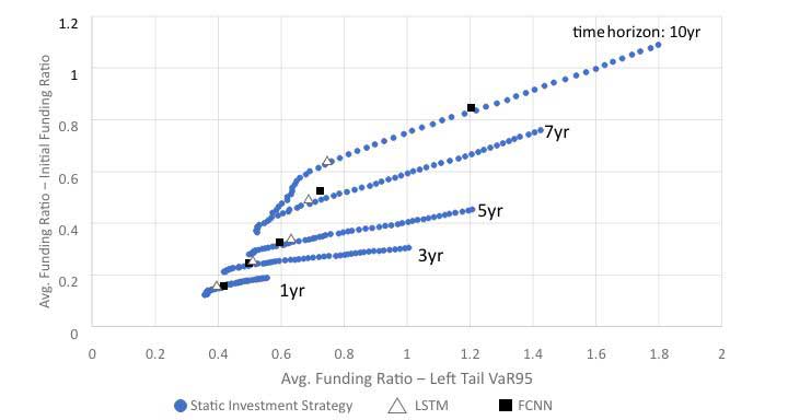
The improvement in risk-return tradeoff occurs when measured across all scenarios rather than within each individual scenario. This means that RL is not trying to enhance gains through market timing, but rather through adjusting asset allocation based on the then-current funding status and economic conditions.
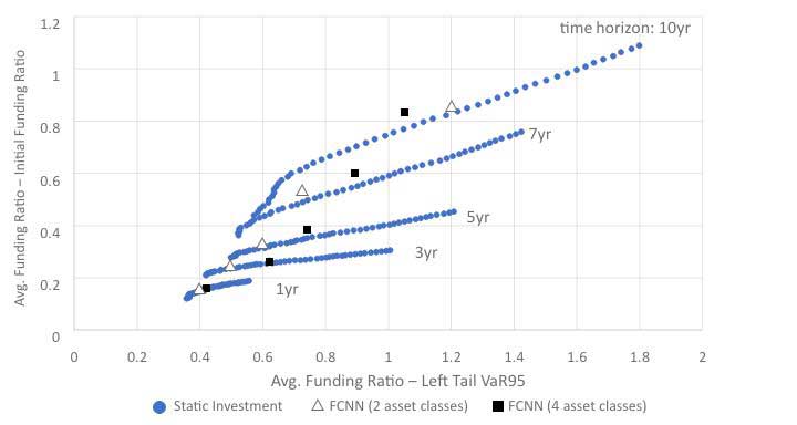
With more asset classes coming into play, it is even more challenging for the traditional approach of LDI strategy optimization because of computational requirements. A test using four asset classes—including AA-rated bonds, BBB-rated bonds, large-cap public equity and real estate investment trusts (REITs)—was performed without updating optimal static investment strategies and efficient frontiers, as shown in Figure 4. An RL-based investment strategy using these four asset classes required less computing time and further improved the risk-return tradeoff achieved with two asset classes.
Figure 4
Dynamic Asset Allocation: Four Asset Classes Without Rebalance Constraint
Overall, this research contributes to the existing literature in three ways. First, it introduces RL and deep learning to actuaries and builds connections with actuarial concepts. Second, it provides a workable example to demonstrate the application of RL to LDI and assess its effectiveness. Without simplifying any liability and asset modeling, it shows the potential of RL to solve complex actuarial problems. The author is not aware of any previous efforts made in this area. Third, sample implementation codes have been made public for educational purposes and can be accessed at https://github.com/society-of-actuaries/Deep-Learning-for-Liability-Driven-Investment.
Statements of fact and opinions expressed herein are those of the individual authors and are not necessarily those of the Society of Actuaries, the editors, or the respective authors’ employers.
Kailan Shang, FSA, ACIA, CFA, PRM, SCJP, is an associate director at Aon PathWise Solutions Group, Canada. Kailan can be reached at klshang81@gmail.com.