
Why Glide Paths Should Evolve
By Dimitry Mindlin
Risk & Rewards, June 2022

What gets us into trouble is not what we don't know.
It's what we know for sure that just ain't so.
Mark Twain
Glide paths find their origins in aviation. A glide path is an aircraft’s evolution in altitude from flying to landing. So, the phrase “evolving glide path” may sound like an oxymoron. In aviation, glide paths evolve by definition.
In investing, “it ain’t necessarily so.” Theoretically, optimal glide paths may be stationary under certain conditions, so glide path evolution requires a rationalization. Most practitioners and academics agree that glide paths should evolve. Most appear to believe they can rationalize glide path evolution. Regrettably, there are good reasons to believe that “it ain’t necessarily so” as well.
The primary objective of this article is twofold. First, it demonstrates that the most popular rationalization for evolving glide paths is flawed and should be discarded. Second, the paper demonstrates that glide paths should generally evolve for investors that endeavor to optimize outcomes and re-evaluate their portfolios regularly. A simplified numerical example illustrates this framework and its assumptions.
Popular Rationalizations for Evolving Glide Paths
“Folk wisdom and casual introspection” suggest the principle “more stocks for the young, more bonds for the old” for glide path evolution. On the surface, the young have more time to weather the volatility of stocks, so the young should invest mostly in stocks and shift to bonds over time. This rationalization is closely related to the controversial “time diversification” property of stocks. Most economists dismiss this rationalization as inadequate.
Economists have long endeavored to rationalize evolving glide paths. Paul Samuelson’s efforts in this area are especially notable. Samuelson (1969) proved that optimal glide paths are stationary (under certain conditions). Later, Samuelson called this result “a failure” because he did not prove that investors “should do something different over time.” Samuelson had recurrently returned to this problem, but the results of these and similar efforts had been lacking.[1]
Despite their importance, these efforts had largely been theoretical prior to the enactment of the Pension Protection Act of 2006 (PPA). The PPA jump-started strong interest in Target Date Funds (TDFs) that promoted glide paths as one of their key advantages. The PPA added a major reason to develop a theoretically sound approach to optimal glide path design.
In April 2007, the Research Foundation of CFA Institute published a monograph Ibbotson (2007). The approach to glide path design presented in the monograph—called human capital theory (HCT)—does rationalize evolving glide paths. The foundation endorsed this monograph as “an unusually complete and theoretically sound compendium of knowledge on this topic.” Today, HCT is broadly accepted in the industry as the core of glide path design.
The trouble is the foundation of HCT is fundamentally flawed.
Human capital is defined as “a capacity to earn income or wages for the remainder of our lives.” Human capital is a series of contingent payments of uncertain magnitude and timing. The main idea of HCT is the assumption that human capital should be treated and priced as a conventional bond-like asset. This assumption is called the pricing assumption in this article.
The pricing assumption has momentous implications. Particularly, the present value of human capital (PVHC) is a known value (a scalar). Few economists or practitioners have challenged or scrutinized this assumption.
The pricing assumption also has major problems. The present value of human capital is calculated before the investment objectives are specified, which makes little sense. Objectives should come first, and suitable present values should follow. Different objectives may require different present values, so present values require careful treatment. Some present values are deterministic, and some are stochastic. The stochastic nature of human capital and its present values is simply “assumed away” in the pricing assumption.[2]
Here is how the pricing assumption rationalizes evolving glide paths. If human capital is a bond, then the total portfolio (the financial capital plus human capital) of the young has a large allocation to bonds. From the portfolio diversification perspective, the young should invest mostly in stocks and shift to bonds as the human capital bond diminishes over time. The trouble is the pricing assumption also necessitates other conclusions that conflict with this principle.
One of these conflicting conclusions is “the order of portfolios in a glide path is irrelevant.” Think of an investor that has made a commitment to contribute fixed percentage p of his income to the retirement plan. The present value of the retirement contributions is equal to p times PVHC. The asset value at retirement (AVR) is equal to the present value of retirement contributions times compounded investment return factors.[3] Therefore, given a glide path with portfolio returns Rk , AVR is equal to the product of percentage p, present value PVHC, and compounded return factors:
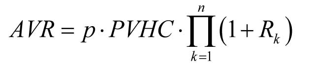 (1)
(1)
According to the pricing assumption, PVHC is a scalar. Since![]() is the same for any transposition of portfolio returns Rk , formula (1) demonstrates that the same is true for AVR. Thus, from the glide path selection perspective, the order of portfolios in the glide path is irrelevant. Obviously, this conclusion conflicts with the principle “more stocks for the young, more bonds for the old.”
is the same for any transposition of portfolio returns Rk , formula (1) demonstrates that the same is true for AVR. Thus, from the glide path selection perspective, the order of portfolios in the glide path is irrelevant. Obviously, this conclusion conflicts with the principle “more stocks for the young, more bonds for the old.”
Furthermore, from the portfolio optimization perspective, some important optimization problems related to AVR in formula (1) lead to stationary glide paths. This is another conflicting conclusion derived from the pricing assumption.
The need for a better approach to glide path design is obvious.
Evolving Glide Paths Rationalized
This section presents a simplified numerical example that demonstrates that the principles “investors endeavor to optimize outcomes” and “investors reevaluate their portfolios regularly” generally lead to evolving glide paths.[4]
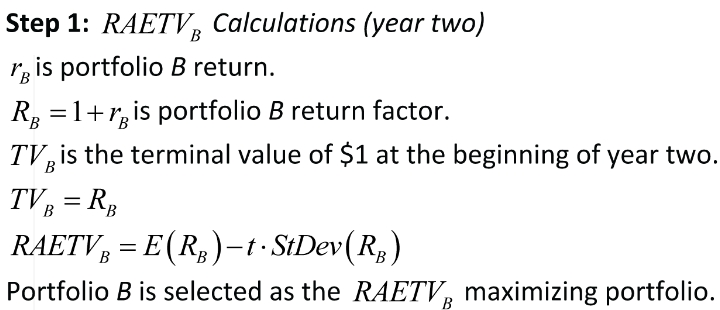
The investor’s commitment is to invest $1 now and $1 in a year. The investor reevaluates his portfolio annually. The key measurement of outcomes is the risk adjusted expected terminal value (RAETV) defined as follows:
RAETV = E − t ∙ S
where the terminal value is the asset value at the end of year two, E is the mean of the terminal value, S is the standard deviation of the terminal value, and t is a risk tolerance parameter. The investor’s goal is to maximize RAETV. Note that the maximization of essentially the same measurement of outcomes is the core of Modern Portfolio Theory.
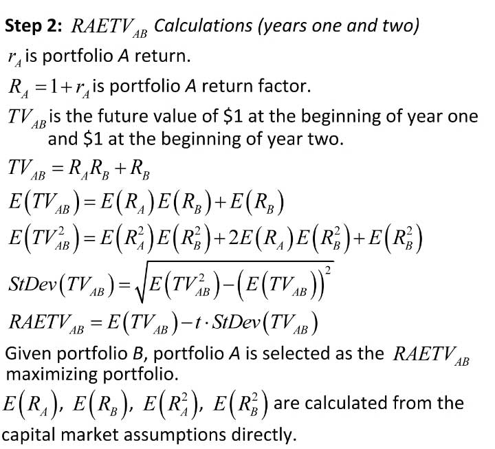
The glide path would have two portfolios: Portfolio A in year one and portfolio B in year two. The annual reevaluation and the RAETV maximization assumptions require that portfolio B would be selected to maximize the second year RAETV. Given portfolio B, portfolio A would be selected to maximize the two-year RAETV. Since the selection of portfolio A depends on portfolio B, portfolio B should be selected first and portfolio A should be selected next. Thus, the assumptions lead to future value maximization via backward induction as the glide path selection procedure.[5] Appendix II contains more technical details about the calculations of RAETV.
For simplicity, we assume that the investor utilizes two asset classes (stocks and bonds) and has the same risk tolerance in years one and two. Appendix I contains the capital market assumptions.
Exhibit 1 presents the stocks allocations for the optimal glide paths for several selected risk tolerance parameters.
Exhibit 1
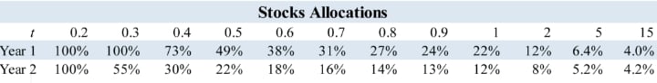
Here is how to read Exhibit 1 for t = 0.5, for example. The RAETV maximizing portfolio in year two is 22 percent/78 percent (stocks/bonds). The 49 percent/51 percent portfolio in year one in conjunction with the 22 percent/78 percent portfolio in year two maximizes RAETV over two years.
Exhibit 1 demonstrates that RAETV maximizing glide paths are evolving.
Here are several additional observations.
- The glide paths in Exhibit 1 are Nash equilibrium solutions.
- The glide paths in Exhibit 1 have the following property: Any sub-glide path of an optimal glide path is optimal on its own. Hence, these glide paths satisfy Bellman's principle of optimality.[6]
- Constant risk in the “asset-commitment” space may imply evolving risk in the “asset-only” space.
- Equity allocations in years one and two can be constant (t = 0.2), decreasing (t = 0.5), or increasing (t = 15).
- The pricing assumption is unnecessary.
Conclusion
The industry must deal with the fact that it has neither a “theoretically sound” approach to glide path design, nor a “theoretically sound” rationalization for evolving glide paths. Clearly, the existing foundation of glide path design requires a major renovation. Without it, millions of investors will continue to utilize inefficient glide paths that generate sub-optimal outcomes. Obviously, this article just scratches the surface. Yet, this author is optimistic that the approach sketched out here presents important initial steps in the direction of a comprehensive optimal glide path design framework that is in the best interests of retirement plan participants.
Statements of fact and opinions expressed herein are those of the individual authors and are not necessarily those of the Society of Actuaries, the newsletter editors, or the respective authors’ employers.
Dimitry Mindlin, ASA, MAAA, Ph.D., president of CDI Advisors, is an investment consultant and an actuary. Dimitry can be contacted at dmindlin@cdiadvisors.com.
Certain aspects of this article may include features disclosed and/or claimed in U.S. Patent No. 8,396,775.
APPENDIX I: Capital Market Assumptions
Return/Risk
| Geometric Mean (%) | Arithmetic Mean (%) | Stanbdard Deviation (%) | |
| Stocks | 7.00 | 8.16 | 16.00 |
| Bonds | 4.00 | 4.12 | 5.00 |
Correlation Matrix
| Stocks | Bonds | |
| Stocks | 1 | 0.2 |
| Bonds | 0.2 | 1 |
Returns in different years are assumed independent.
APPENDIX II: Terminal Value Calculations
References
Bellman, R.E. (1957), Dynamic Programming, Dover.
Ibbotson, R., Milevsky, M., Chen P., Zhu, K. (2007). Lifetime Financial Advice: Human Capital, Asset Allocation, and Insurance, The Research Foundation of CFA Institute.
Mindlin, D., (2013). A Tale of Three Epiphanies, CDI Advisors Research, CDI Advisors LLC.
Mindlin, D., (2022). A Tale of Two “Scandals,” CDI Advisors Research, CDI Advisors LLC, forthcoming.
Samuelson, P., (1969). Lifetime portfolio selection by dynamic stochastic programming, The Review of Economics and Statistics, 51, 239-246.
Samuelson, P., (1989). A Case At Last for Age-Phased Reduction in Equity, Proc. Natl. Acad. Sci. USA, Vol. 86, 9048-9051.
Samuelson, P. (1992). At Last, a Rational Case for Long-Horizon Risk Tolerance and for Asset-Allocation Timing? Active Asset Allocation, edited by Arnott, R.D. and Fabozzi, F.J., Probus Publishing Company.