
Low Interest Rates and the NAIC Economic Scenario Generator Project
By Stephen J. Strommen
Risk & Rewards, June 2022

The valuation of insurance liabilities for accounting purposes has evolved in the 21st century so that it is often based on stochastic simulation and discounting of future cash flows in an asset-liability simulation model. In the U.S. such valuation methods have been called “principle-based” and are encoded by the NAIC in the Valuation Manual for use in required regulatory financial reporting, especially for long-term insurance contracts with guarantees that involve investment risk. Internationally, a different new standard of accounting for insurance contracts (IFRS 17) also employs such stochastic asset-liability simulation methods for valuation, but with important differences.
Stochastic asset-liability simulation methods require use of a stochastic economic scenario generator (ESG). There are many formulations of such a generator, but for regulatory purposes the NAIC mandates a particular one. The NAIC is working on a project to replace the ESG that it mandates be used for these regulatory reporting requirements. One of the main reasons for doing so is that interest rates in the market wandered outside the range that the current ESG could produce. Short-term interest rates fell to zero, while the current ESG has a floor above zero.
Another reason for replacing the ESG is that the American Academy of Actuaries (the Academy), which created and had been maintaining the ESG, made it clear that another party should take over maintenance of the ESG used for regulatory purposes. There are several reasons for that, but they are beyond the scope of this article.
The NAIC decided to contract with a private firm to provide its ESG. They selected Conning, and Conning’s interest rate generator is based on a three-factor Cox-Ingersoll-Ross (CIR) model. It has become clear that some modification of that model is needed to make it suitable for NAIC purposes. This article explains why such modification is needed and outlines two approaches that are under consideration.
Understanding the Three-factor CIR Model
The three-factor CIR model is just the sum of three one-factor CIR models, each with different mean reversion parameters and volatility. The sum of three allows the model to reproduce a wide variety of yield curve shapes. But the general distribution of the level of future interest rates is still much like that in a one-factor CIR model, and the issue with low interest rates can be understood in that context.
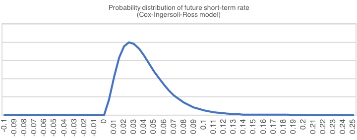
A one-factor CIR model is a simple mean-reverting random walk. The unique aspect of the CIR approach, as compared to other models like Vasicek, is the volatility. In a CIR model, volatility is proportional to the square root of the short-term interest rate. That means that when the interest rate approaches zero, the volatility approaches zero and the mean reversion term dominates. In a continuous version of the model this prevents interest rates from ever going below zero. The result is a distribution of interest rates in the far future that is skewed and looks something like Figure 1:
Figure 1
Probability Distribution of Future Short-term Rate (Cox-Ingersoll-Ross Model)
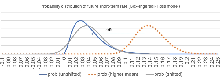
One of the features the NAIC wanted in a generator was the possibility of producing negative interest rates. Clearly, a traditional CIR model cannot do that. But Conning’s version adds another parameter to enable a CIR model to produce negative interest rates. The extra parameter is a “shift.” This is simply a number that is subtracted from all short-term rates produced by the model. When a shift is included, one can set the mean reversion point higher so that the distribution of interest rates before the shift is higher, but the minimum is still zero. When the shift is subtracted, the distribution is re-centered around normal levels, but the minimum is not zero, it is negative by the amount of the shift. Mathematically, this change also has the effect of reducing the skewness of the distribution of future interest rates so that it more closely resembles the Gaussian bell-shaped curve. (See Figure 2)
Figure 2
Probability Distribution of Future Short-term Rate (Cox-Ingersoll-Ross Model)
It turns out that the size of the shift plays a significant role in the ability of the three-factor CIR model to fit a variety of yield curve shapes. Good fitting requires a significant shift on the order of 10 percent or more. And that’s where the problem comes in. With a significant shift, the future distribution is not as skewed and the likelihood of interest rates far below zero becomes significant.
When the shifted CIR model is calibrated with a mean reversion point specified by the NAIC and with reasonable volatility at the mean and mean reversion speed, one gets a distribution of future interest rates that is shaped more like a bell-shaped curve. If the mean reversion point is 4 percent, then it is almost equally likely that interest rates could be +/– 5 percent from there. That makes future interest rates of -1 percent and 9 percent almost equally likely and assigns significant probability to rates down to -3 percent and lower and up to 11 percent or more. That’s the problem—most people, including regulators, do not find it reasonable to model interest rates so far below zero or so frequently below zero. Therefore, the model needs adjustment to be suitable for this purpose.
Adjusting the Model
Fundamentally, the task at hand is to adjust the distribution of future interest rates to make it more skewed, that is, reduce the frequency and severity of negative interest rates. The mean reversion point is much closer to the bottom than the top of the realistic range of future interest rates, based on historical behavior. The shifted CIR model does not produce such a skewed distribution. So, what can be done?
A complete replacement of the model is one obvious choice. But the NAIC has already contracted with Conning, apparently before learning of these issues. For the remainder of this article we will explain two methods that have been proposed to address this issue within the context of the three-factor CIR as the model to be used.
The two methods under consideration both grew from the idea of a simple floor. One could simply adjust the model by setting any generated interest rate below zero to zero. A simple floor at zero was rejected for two reasons.
- Regulators wanted a material possibility that interest rates could fall below zero.
- The frequency with which future interest rates would be floored at zero was viewed by subject-matter-experts (SMEs) as unreasonably high. The flooring at zero would not be a rare event, it would happen frequently.
A method was desired that would both allow for some negative interest rates while at the same time decreasing the frequency of zero or negative interest rates. The concept of a “Generalized Fractional Floor” (GFF) was developed to accomplish that.
The Generalized Fractional Floor
A Generalized Fractional Floor has two parameters: A threshold and a fraction. The threshold acts as a kind of soft floor. Any generated rate below the threshold is adjusted. The adjustment reduces the distance below the threshold to a fraction of its original value. This compresses the distribution of generated rates below the threshold. Basically, it squeezes the distribution of the lower tail into a smaller space.
The following formulas are used:
T = Threshold
F = Fraction
O = Observed rate (the adjusted generated rate) = T – F(T – S) when S < T, otherwise O = S
S = Generated rate (“shadow rate”) = T – (T – O)/F when O < T, otherwise S = O
When using these formulas, any rate below the threshold produced by the unadjusted ESG is adjusted upwards to produce the “observed” rate, that is, the rate included in the adjusted scenarios. The output of the ESG is the adjusted “observed” rates. When the threshold is above zero and the fraction is less than 1.0, this reduces both the frequency and severity of negative interest rates.
This approach creates an issue when the starting observed rate is below the threshold. The adjusted value of the starting rate must be the observed starting rate. That means that whenever actual starting rates are below the threshold the starting conditions fed into the ESG must be different from the actual observed starting conditions. In the formulas above, the value of “O” is the observed rate and the value of “S” is the value to be used in the initial yield curve for the generator.
The starting conditions adjusted in this manner have been called “shadow rates.” The ESG becomes a model for generating scenarios of shadow rates. Scenarios of observed rates are obtained by applying the GFF formulas to all the yield curves in the scenarios of shadow rates.
Discussion so far has focused on the short-term rate. The GFF approach seems reasonable when applied to just the short-term rate. But an ESG produces full yield curves. The GFF approach can be applied to the entire yield curve, using the same threshold and fraction for every maturity. But this often creates a “kink” or abrupt bend in the yield curve at the level of the threshold value. The slope abruptly changes at that point; it is multiplied by the fraction “F” which may be on the order of 20 percent. The resulting adjusted yield curves are not arbitrage-free, even when the underlying model for shadow rates is arbitrage-free. The three-factor CIR model is arbitrage-free before this kind of adjustment but not after.
The Shadow Rate Floor
It is possible to employ the shadow rate concept in an arbitrage-free manner so that the resulting scenarios are arbitrage-free both before and after the adjustment and there is no “kink” in the adjusted yield curve. That’s what is done in what is being called the Shadow Rate Floor (SRF). The difference from the GFF is in how the yield curve is completed based on the model for the short-term rate.
In both the GFF and the SRF, completion of the yield curve involves a fundamental formula commonly used to determine spot prices using the risk-neutral calibration of an arbitrage-free model.[1] The spot price is the expected present value of a future payment using path-wise discounting at the short-term rate.

In the three-factor CIR model, there is a closed form expression for this expectation. That closed form expression is used to compute the yield curve at any time step starting with the short-term rate. When applying the GFF, the yield curve that is computed using this formula is the shadow curve. Each point on the shadow curve is then adjusted using the GFF formulas, and that can result in yield curves with a kink at the threshold value.
The concept of the Shadow Rate Floor is to use the GFF to modify the path of the short-term rate, and then use the formula above to complete the yield curve using the modified expectation of the path for the short-term rate. The concept is simple, but in practice this is complicated by the fact that when the path of the short-term rate is modified this way there is no longer any closed-form expression for the expectation in the formula for the spot price shown above. Spot prices based on that expectation need to be estimated through stochastic simulation.
Use of a stochastic simulation to complete each yield curve in a set of stochastic scenarios is impractical. Fortunately, it was discovered that a reasonably good approximation exists in this case. The approximation is to complete the shadow curve in the same manner as is done in the GFF (that is, using the closed form expression in the three-factor CIR model), but then adjust it with a table of factors that varies by term to maturity. Where the GFF uses one threshold and fraction to adjust all points on the yield curve, the approximate shadow rate floor uses a different threshold and fraction for each point on the yield curve.
Table 1, below, is based on a threshold of 0.40 percent and a fraction of 20 percent for the short-term rate and one reasonable calibration for the three-factor CIR model. For brevity, values are shown for only a few terms to maturity.
Table 1
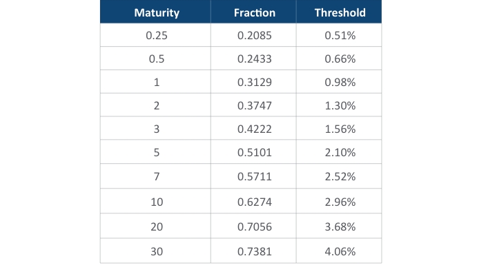
A table like this provides a practical means to make a good approximation to the yield curve with a shadow rate floor. The table results from a complex estimation process involving both stochastic simulation and regression. The values in the table depend on both the parameter values used in the three-factor CIR model and on the threshold and fraction that define the GFF applied to the short-term rate. Since both the parameters and the definition of the floor are unlikely to change very often, the table would not require frequent updates.
Note that the threshold values in the table increase with term to maturity. Whereas the short-term rate is only adjusted by the floor if it is under 0.40 percent, the 20-year rate is adjusted if it is under 3.68 percent. If the 20-year shadow rate produced by the three-factor CIR generator is between 0.40 percent and 3.68 percent then it would be adjusted using the SRF but would not be adjusted using the GFF. This means, in general, that the long end of the yield curve tends to be higher under the SRF when interest rates are generally low. Conversely, it means that the starting curve used to initialize the three-factor CIR model (the shadow curve) when using the SRF is always less than or equal to that when using the GFF.
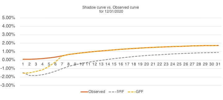
Figure 3, below, shows the 12/31/2020 observed curve and the shadow rate curves used to initialize the generator when using the GFF and the SRF. The floor on the short-term rate uses a threshold of 0.40 percent and a fraction of 20 percent in both cases.
Figure 3
Shadow Curve Versus Observed Curve for 12/31/2020
The NAIC is still in the process of reviewing and testing the proposed new ESG. It is not certain that either of the approaches discussed in this article will be adopted. Some observers find both to be less than satisfactory and other approaches are possible. Nevertheless, the behavior of the generator at low interest rates is likely to remain a focus of attention.
Statements of fact and opinions expressed herein are those of the individual authors and are not necessarily those of the Society of Actuaries, the newsletter editors, or the respective authors’ employers.
Stephen J. Strommen, FSA, CERA, MAAA, is an independent consultant, owner of Blufftop LLC, and member of the AAA Economic Scenario Generator Work Group. Stephen can be contacted at stevestrommen@blufftop.com.