
Fixed Indexed Annuity Fair Value Quantification and Valuation
By Peter M. Phillips and Tao Wang
Risk Management, February 2022

The Accounting Standards Update (ASU) 2018-12 (titled “Targeted Improvements to the Accounting for Long-Duration Contracts”) issued by the US Financial Accounting Standards Board (FASB) aims to improve the disclosure requirements under US GAAP for certain long-duration contracts including FIA products. One of the areas of focus within ASU 2018-12 is the reporting of a new market risk benefit (MRB) classification of liabilities, which must be valued in a market-consistent way following LDTI requirements. Guaranteed minimum living and death benefit riders offered in fixed index annuity (FIA) products are typically valued and reported using risk-neutral scenarios.
Coincidentally, the draft principle-based reserving (PBR) framework for FIA products (VM-22) by the National Association of Insurance Commissioners (NAIC) introduces a stochastic reserve component similar to what VM-21 requires for variable annuity products. The transition from the current deterministic framework to VM-22 is a challenge for many insurers, but also provides opportunities to measure and manage risks in FIA products in a more consistent way.
In this article, a numerical comparison of two commonly used FIA valuation methodologies is conducted to help insurers decide on the best methodology to use under GAAP LDTI and VM-22. We compared two modeling approaches to project the future index credits with the annual point-to-point crediting formula: The stochastic equity crediting model and the deterministic option budget crediting model. The analysis is then extended to different levels of option budgets and the monthly average crediting formula. The advantages and disadvantages of the two equity return projecting approaches are also highlighted and will be discussed later in the report.
We conclude that the stochastic equity crediting model is more capable of capturing the fair value of the FIA riders across the two crediting methods and different assumption settings. The valuation of the embedded guarantees involves complex mathematics and requires sophisticated stochastic-on-stochastic (SoS) simulations. The option budget crediting model is a shortcut approach that can produce material discrepancies in some situations compared to the more robust stochastic equity crediting model. Furthermore, the option budget crediting model produces a single best estimate rather than a distribution required for PBR reserving and risk management purposes.
Approaches, Data and Assumptions
Two approaches are commonly used to project index credits: The stochastic equity crediting and the deterministic option budget crediting.
- Stochastic Equity Crediting. The model requires a market-calibrated stochastic equity simulation model to generate a large number of equity scenarios under risk-neutral settings. The algorithm also calculates option prices (with different strike prices) for each simulated scenario. Based on these prices and the available option budget level, we can then calculate the resulting cap rate, participation rate and index spread. These parameters are reset at the beginning of each year and are held constant throughout the year. After applying the parameters to the index change, we will arrive at the indexed return under the stochastic equity crediting model. This model is sophisticated and requires a state-of-the-art simulation model and computational resources.
- Deterministic Option Budget Crediting. The model is a shortcut model that does not require simulation of equity returns. Crediting the account value is simply based on the available option budget level. At the beginning of each year, the model records the available option budget level and then accumulates the available option budget level at the risk-free rates during the year. To allow it to be comparable to the stochastic equity model, the crediting rate does not fall below a floor rate that corresponds to the minimum cap rate, and the floor rate is backed out by the Black-Scholes formula. This approach is fast and simple. One immediate disadvantage of this approach is that it does not capture the full distribution of the results for tail risk management and reserving purposes.
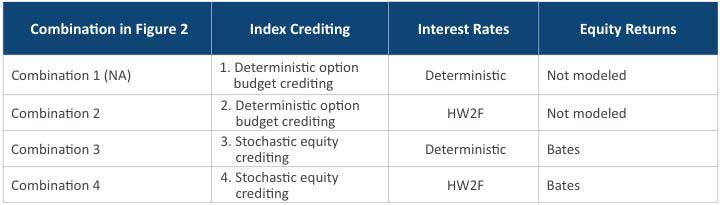
To see which approach is more capable of capturing the fair value of MRB, we compared results under four different models, starting from the simplest (deterministic option budget crediting model with deterministic interest rate model) to the most complex one (stochastic equity crediting model with stochastic interest rate model), as listed in Table 1.
Table 1
MRB Valuation Model Specification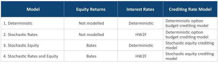
For risk-neutral equity simulations, the Bates model is used. Compared to the traditional Black-Scholes framework, the Bates model is capable of simulating both stochastic volatilities and stochastic jumps. The Bates model is one of the sophisticated market risk models used today by FIA insurers. For interest rates simulations, the Hull-White 2-Factor (HW2F) short rate model is used to capture non-parallel movements of the yield curve and can produce a more realistic interest rate volatility term structure. In our analysis, both models were calibrated to the prevailing capital market environment to generate market-consistent results.
To set the available option budget level, we follow the common practice of taking the difference between the general account yield and the required pricing spread. The general account yields are simulated. However, the required pricing spread is a more subjective assumption, as it depends on the insurer’s profitability expectation. Therefore, in order to remain unbiased, we performed result comparisons on different levels of required pricing spreads.
Dynamic lapse is also important risk to reflect in FIA analysis. A policyholder’s surrender incentive depends on the moneyness of a policy. It is assumed that a policyholder rationally compares the present value of expected benefits to the surrender value when making surrender decisions. When the surrender value is sufficiently higher than the present value of expected benefits, the policyholder will have a higher incentive to lapse the policy. Dynamic lapse rate varies across different simulated interest rate and equity return scenarios.
Another important consideration in this analysis is available option budget level. It can be modeled as the difference between the general account yield and the required pricing spread. The general account yield depends on the investment performance of a designated investment portfolio that is mostly comprised of fixed income assets. The required pricing spread is set by the insurers to meet profitability requirements. Within the available option budget, insurers typically execute a 1-year strategy to hedge the crediting rate guarantees. Because the option prices and the general account yield fluctuate, the parameters of the options are reset annually.
With a higher level of available option budget, the cap on indexed return can be set higher, as illustrated in Figure 1. When the available option budget level is below a certain threshold, the cap rate stays at its minimum level.
Figure 1
Cap Rate Versus the Available Option Budget Level
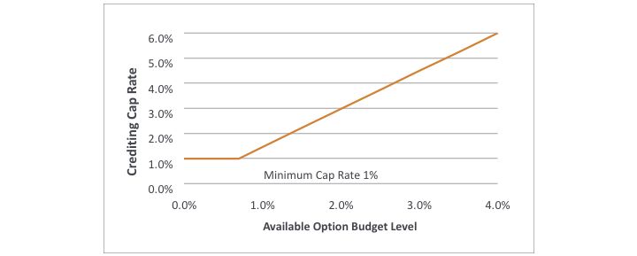
Table 2 lists the sample FIA portfolio used in our analysis. All the policies have an annual reset cap strategy, guaranteed lifetime withdrawal benefit (GLWB) and guaranteed minimum death benefit (GMDB) riders. The resetting cap rate never falls below 1.00 percent, in other words, the minimum cap rate is 1.00 percent. The benefit base for the illustrated GLWB rider has an annual roll-up between 6.50 percent and 7.00 percent (depending on the rider chosen by the policyholder) compounding annually until activation of the benefit. The annual rider fee ranges between 0.95 percent and 1.10 percent of the benefit base. The annual maximum withdrawal percentage depends on the policyholder’s attained age at activation of withdrawals and whether the FIA contract is a joint policy.
Table 2
In-force Policy Book Profile

Assumptions
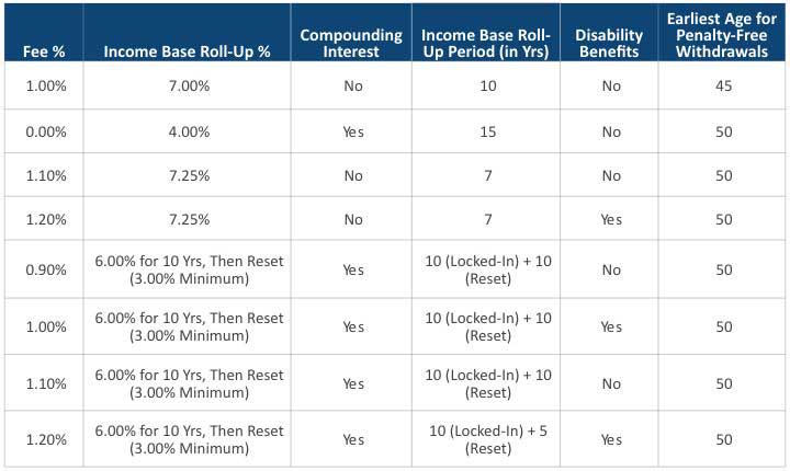
We compared the rider fee assumption as listed in Table 3 against industry observations as listed in Table 4 to ensure realistic parameters were used in our analysis. For each policy, one of the rider fee structures is used.
Table 3
Rider Fee Assumptions
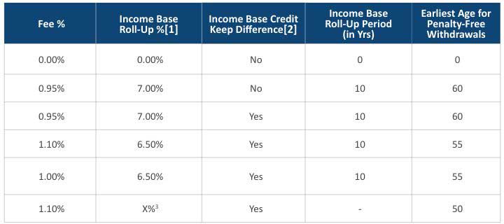
Notes:
- Income base roll-up is compounded annually.
- This feature provides flexibility to the policyholders. During the income base crediting phase, when there is a small amount of withdrawal, the income base will be credited by the difference between the income base roll-up percentage and the withdrawal percentage.
- If withdrawals already happened, roll-up rate = 1.5 × account value growth. Otherwise, the roll-up rate = 2.5 × account value growth.
Table 4
Typical Rider Fees
Baseline Analysis: Annual Point-to-Point Crediting Method
The indexed crediting on the policy account value depends on both the performance of an external index (such as S&P 500®) and the account value crediting method chosen. The performance of the policy account value has a direct impact on the MRB.
The annual point-to-point method is the most common type of crediting in FIA markets. The index change depends only on the difference between the equity index end point and its starting point and ignores the points in-between. The index change using this method is calculated as follows:
![]()
To arrive at the indexed return, an index spread is deducted from the index change, and the difference is multiplied by a participation rate that defines the portion of the gain in the stock index to be credited. The indexed interest rate is subject to a cap rate and never falls below 0 percent.
![]()
The insurance company has the right to periodically reset the indexed return parameters, which mainly depend on the fluctuating available option budget level. With varying pricing spreads and shocks to general account yields, the performance of the four models is listed below.
1 Percent Pricing Spread
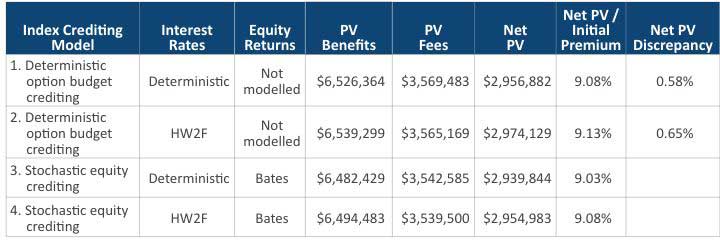
Table 5 below presents the results across four model combinations in Table 1. The “PV Benefits” column in the table quantifies the actuarial present values of the insurance company’s future market risk liabilities using the models specified in each row. The “Net PV” column presents the fair value result which is the difference in present values between the future benefits and ascribed fees. The last column “Option Budget Approach Discrepancy” compares the result of the deterministic option budget crediting model with the stochastic equity option budget crediting model given the same interest rate model.
Table 5
Results (Pricing Spread = 1%)
Notes:
- PV Benefits: Actuarial present values of the insurance company’s future market risk liabilities using the models specified in each row.
- Net PV: Fair value of the difference between the future benefits and ascribed fees.
- Net PV Discrepancy due to option budget approach: Difference between deterministic option budget crediting approach and the stochastic equity option budget crediting approach given the same interest rate model. $2,956,882 / $2,939,844 – 1 = 0.58% and $2,974,129 / $2,954,983 – 1 = 0.65%.
With a 1 percent pricing spread, there is no material difference among the models. However, the situation changes with different general account yield assumptions. Table 6 shows the results with the same pricing spread but a parallel shift of the general account yield curves up by 1 percent. It provides a higher level of option budget than the prior case and is plausible during a rising interest rate environment. The deterministic option budget crediting model underestimates the liabilities by more than 12 percent in comparison to the stochastic equity crediting model and fails to capture the full dynamics of the equity scenarios.
1 Percent Pricing Spread and Parallel Shift Up General Account Yield by 1 Percent
Table 6
Results (Pricing Spread = 1 Percent and Shift Up General Account Yield by 1 Percent)

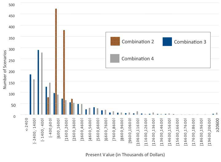
All model combinations but the first one (a deterministic interest rate model with equity return not modeled) are able to produce present value distributions. Figure 2 shows the different distributions. We see a material impact of the interest rate model on the distribution of the present values. Therefore, model selection is important when it comes to managing the product risk across a wide range of scenarios, especially in extreme scenarios. The deterministic modeling approach is insufficient in this case.
Figure 2
Net PV Histogram Across Combinations in Table 6
Note:
2 Percent Pricing Spread
The pricing spread can also make a big difference among model results, as shown in Table 7. The interest rate model was calibrated to the market prices observed in December 2019 when the 10-year US Treasury yield was below 2 percent. If the insurer requires a relatively aggressive pricing spread of 2 percent under such an interest rate environment, the available option budget level will be low and even reach 0 percent for some simulated scenarios.
When the available option budget level is 0 percent, the minimum cap rate guarantee will be activated. In other words, the cap rate will stay at the minimum 1 percent level.
- Under the stochastic equity crediting model, the account value will be credited using a bull spread option strategy with a floor of 0 percent and a cap of 1 percent.
- Under the deterministic option budget crediting model, the account value will be credited directly by the price of this bull spread option strategy. Because there is no equity simulation involved in this model, by default, the pricing is produced by the Black-Scholes formula.
Table 7
Results (Pricing Spread = 2 Percent)
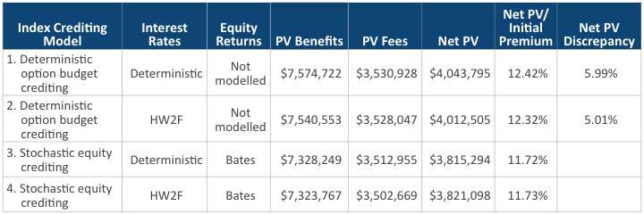
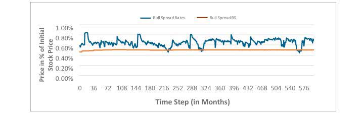
In this case, the deterministic option budget crediting model overestimates the liabilities by more than 5 percent. The Black-Scholes formula does not capture the stochastic nature of volatilities and jumps. Therefore, it undervalues the bull spread option strategy under most scenarios. Figure 3 compares the prices simulated by the Bates model to the Black-Scholes prices under a typical interest rate scenario:
Figure 3
Bull Spread Option Strategy Price Comparison between Bates and Black-Scholes (BS)
Extended Analysis: Monthly Average Crediting Method
To investigate the impact of different crediting methods, the comparison of the four model combinations is extended to the monthly average crediting method. The monthly average crediting method records the values of a stock index at the end of each month, then takes the average of 12 consecutive month-end index values to get the 12-month rolling average. This crediting method compares this 12-month rolling average to the index value at the beginning of the year to determine the index change, as specified below.
![]()
Compared to the annual point-to-point crediting method, this crediting method reduces the index volatility by averaging the index values and has a limited upside potential. On the modeling side, the path dependent nature of this crediting method is more challenging to handle. Indexed returns are determined using the same rule as in the annual point-to-point crediting method. The insurance company has the right to reset the parameters including the cap rates, the participation rates and the index spreads based on available option budget.
Table 8 shows the results with a pricing spread of 1 percent.
Table 8
Results (Pricing Spread = 1 Percent)

Similar to the annual point-to-point crediting method, no material difference is observed when the pricing spread is 1 percent. Table 9 shows the results with a 1 percent parallel shift of the general account yields. The deterministic option budget crediting model underestimates the liabilities by more than 20 percent in comparison to its stochastic counterpart, similar to what we observed in the annual point-to-point crediting method.
Table 9
Results (Pricing Spread = 1 Percent and Upward Shift General Account Yield by 1 Percent)

Conclusion
The deterministic option budget crediting model produces a simple best-estimate valuation and is faster to compute. But we observed this shortcut model can significantly underestimate or overestimate the FIA liabilities, compared to stochastic models that use a large number of market-consistent equity return scenarios. It also fails to capture the entire distribution of valuations, which is important for risk management.
The MRB reporting introduced by ASU No. 2018-12 generally requires FIA riders to be reported at fair value post LDTI. Additionally, under the newly introduced PBR framework for fixed annuities (VM-22), reserving for FIAs riders will likely require the use of a CTE 70 measure. While evaluating various modeling approaches to meet new regulatory requirements is important, it is also a good opportunity to consider how the models can help quantify risks in FIA products.
Statements of fact and opinions expressed herein are those of the individual authors and are not necessarily those of the Society of Actuaries, the newsletter editors, or the respective authors’ employers.
Peter M. Phillips, is president and CEO for Aon PathWise Solutions Group LLC. Peter can be contacted at peter.phillips@aon.com. LinkedIn.
Tao Wang, Ph.D., ASA, MAAA, is managing director and head of consulting solutions forAon PathWise Solutions Group LLC. Tao can be contacted at tao.wang@aon.com. LinkedIn.