
Challenges of Managing Interest Rate Risk: Part 1—How to get the Most Insight out of a Company's Assets and Liabilities
By Dariush Akhtari
Risk Management, February 2024

The mismatch between how interest rate impacts the value of assets and liabilities could have material negative impact to companies’ earnings and surplus. To quantify and mitigate the impact of such mismatches, companies have used matching a combination of duration and convexity. In this part of this multipart paper, I will review these measurement techniques and their limitations. The next part will provide an approach to better understand to what extent these measures could be relied on and how to extend their use.
To mitigate interest-rate risk, it is imperative to match the characteristics of assets to those of liabilities. The mismatch between how interest rate impacts the value of assets and liabilities can have material negative impact on companies’ earnings and surplus. An example is Q1 2020 when the spot curve dropped between 138 bps to 87 bps (for years one to 30). Quantifying and attempting to mitigate its impact on surplus requires well-designed models projecting asset and liability cash flows. Historically, this was achieved by matching duration or matching the duration and convexity of the assets to those of the liabilities. However, these techniques are only suitable to immunize interest-rate risk for small and parallel movements. In this part, a simple example is used to highlight that even with parallel rate change these metrics have limitations. In Part 2 of this article series, I will provide a method to identify the range of rate changes where these ALM metrics may be relied upon, the “validity” range, outside of which recalculation of the ALM metrics may be required in addition to potential need for rebalancing the portfolio. Additionally, in Part 2, I will provide a technique to improve on the approximation of value change outside of the aforementioned “validity range.”
Review of Various Measurement Techniques and Their Limitations
Many are familiar with ALM metrics duration and convexity. However, to mitigate the risk of impact to surplus (value of assets less the value of liabilities) after a rate change by matching of duration and convexity of assets and liabilities requires having asset value to be equal to the liability value. This point can be lost on many, but it is crucial. A solution to this problem is to match “discounted value” or “dollar value,” DV01, and “dollar convexity value” of 1 basis point, CV01, of assets and liabilities.
DV01 stands for discounted value or dollar value of 1 bp increase to the interest rate curve. It is equal to the negative of the product of duration and market value of the instrument divided by 10,000. CV01 stands for dollar convexity of the instrument for a 1 bp change to the interest rate curve. It is equal to the product of convexity and market value of the instrument divided by 100,000,000. The advantage of matching DV01 and CV01 of assets and liabilities is that it is not needed to have the restriction of value of assets being equal to that of liabilities. The value change to the instrument for a parallel shift in a basis point of h would then be:

Note that DV01 of a bond is negative since a rate increase decreases the value of the bond.
In this article I will refer to any or all the above as asset and liability management (ALM) metrics or simply metrics.
Illustration of Challenges with the above Metrics Using GIC
I will use a simple guaranteed investment contract (GIC) example to illustrate the limitations and challenges experienced by the above measures.
How Shifts are Applied for the Calculation of the Metrics
To reduce interest-rate risk, a basket of assets is chosen that have ALM metrics matching those of liabilities. For the calculation of ALM metrics, one would shift the entire interest rate curve by a small change in rates (say 10 bps) up or down. Below I will discuss shift size and its implications. In finance, many use a shift size of 25 bps to 50 bps. One rationale for using a large shift size is that since the calculated metrics are further used for approximations of impact of value due to rate change, a higher shift size would mitigate the extrapolation implied using the metrics for rate changes beyond the shift size. Another reason for using larger shifts may have stemmed from the fact that many only used duration-matching (i.e., did not use convexity), and thus, wished to capture some element of convexity change in the first order approximation.
Situations where ALM Metrics Provide Less Reliable Forecasts
The volatility of cash flows around the inflection points will limit the effectiveness of using ALM metrics to forecast changes in liability values.
Size of the Shift
It should be noted that DV01 is the slope of the tangent lines to the graph of the value at the rates when a shift size close to zero (1 bp or less) is used. When the shift size is larger, they represent the slope of the cord connecting values created by +/- shift to the rates.
To examine this further, I work with a simple example. Let’s assume we have a simple GIC contract with $1,000 account value, 3% minimum guarantee rate, 2% profit margin, and 10% partial withdrawal per year projected for 30 years at which point the contract is fully surrendered. Spot rates are assumed level for this simple example.
From Figure 1, it can be noted that there is a point of inflection at 5% (3% minimum guarantee rate + 2% profit margin) after which the expected profits are fixed at 2% of the account value. Note that the convexity of the value changes from negative to positive at 5% as can be seen in the graphs in Figure 1 below. The second and third graphs are the same graph as the first however, they have been zoomed in to reflect values using flat spot rates below 5% and above 5% with a fitted quadratic polynomial to the graphs to highlight the change in convexity.
Figure 1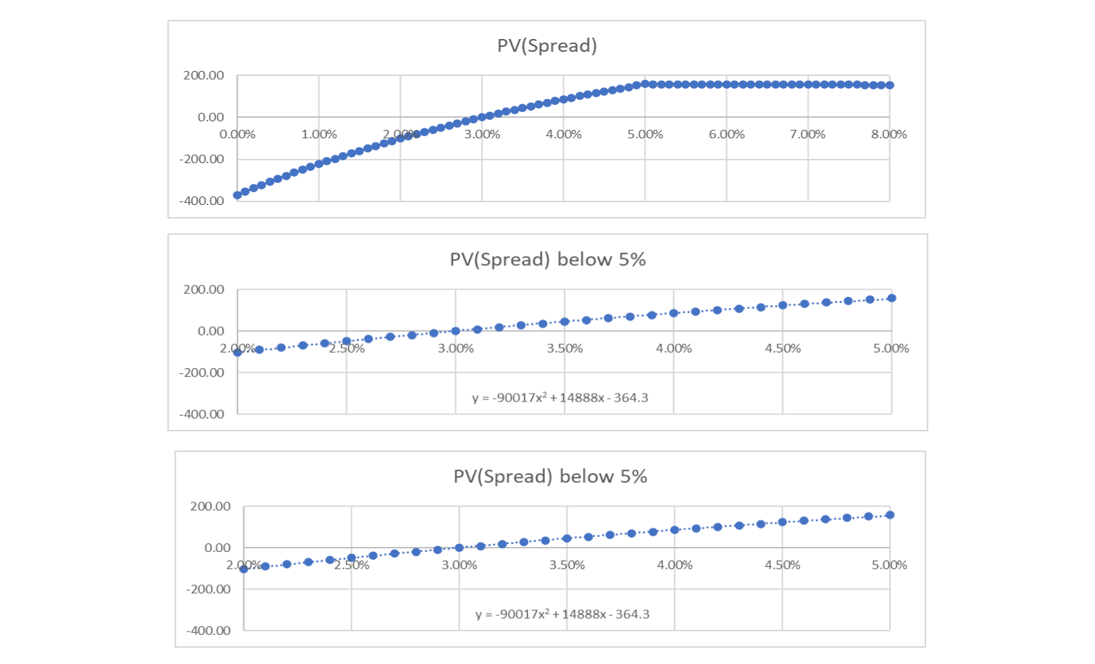
A point on the graph plus its adjacent points, represent value at the point and those used in the calculation of the up and down shifts that will produce the DV01 and CV01.
Note the sign of the coefficient of x2 in the fitted curve (sign of convexity) to the value changes from negative to positive at 5%, making 5% a point of inflection. This is important since when DV01 & CV01 are used to estimate the value change after a shift, it is assumed that the value continues along the quadratic function fitted to the three values calculated at the spot rate and the spot rate plus and minus the shift. The importance of this becomes clear below.
Let’s initially consider the shift to be very small so that the spot rate and spot rate plus and minus the shift all are on one side of the inflection point. Then the best approximation using DV01 and CV01 calculates using these points can only be reasonably accurate for approximations that are applied to changes in rate that are less than or equal to the difference between the point of inflection and the current spot rate. To give a numeric example with our example, let’s assume the current spot rate is 4.5% and DV01 and CV01 have been calculated using a 10-bp shift. The approximation of value for an increase in rates is most accurate for up to 50 bps (5% - 4.5%). The approximation using shifts of higher than 50 bps are less trustworthy, and the calculated value could be coincidentally close or dramatically different than the actual value depending on the level of the change in the convexity after the inflection point and the level of the rate change that is in excess of 50 bps. This can be seen in Tables 1 to 3 below under the second column (4.5%). Note that regardless of the shift level (1, 10, and 50 bps), the approximation is quite accurate for a rate increase of 30 bps (getting to 4.8%, which is below 5% where the point of inflection occurs). However, the approximation is no longer accurate with a 75 bp change where the resulting rate is 5.25% (past the inflection point).
Now let’s consider when the shift level puts the calculation points on opposite sides of the inflection point. For example, current spot rate is 4.95% and a shift size of 10 bps is used. This means that the quadratic function to be used in the calculation of DV01 and CV01 (used for the approximation of value for rate change) is fitted to values at 4.85%, 4.95%, and 5.05%. Note that two of these points lie below the inflection point and one above. This will produce a function with negative convexity where its maximum value is achieved below 5.05%. Any approximation for rates in excess of 5.05% is not trustworthy since for an increase in rate, the approximation will produce a value that would be below the actual (note that post 5%, the convexity of the graph of value against spot turns positive with much smaller magnitude). This can be seen in Tables 1 to 3 below under the third column (4.95%). Both the 30 bp and 75 bp shifts produce bad approximations regardless of the shift size. It should be noted that the approximation inaccuracy using a shift size of 50 bps is less severe simply because more of the post 5% value gets used in the calculation of DV01/CV01. However, had we calculated a rate decrease (say -30 bps or -75 bps), the approximation using a 50bp shift would have produced worse results since more of the calculated values were based on values below 5%.
If one wants to ensure that the three points used in the calculation of DV01 and CV01 stay on one side of the inflection point, it seems that it is best to have the shift size to be as small as possible, say 1 bp. In fact, looking at Table 1 when the spot rate is at 4% using the combination of DV01 and CV01 can produce extremely good approximation even at a 75 bp rate increase (55.65 vs. 55.83). Note the 4.75% is still less than 5%. However, using the same 1 bp shift when the rate is at 4.5% does not produce as good an approximation with rates increasing by 75 bps to 5.25% (51.52 vs. 34.78). The situation worsens when the current rate is at 4.95%. Even an increase of 30 bps to 5.25% produces a bad approximation (19.96 vs. 3.06). However, once current rates are past the 5.5% ensuring all the rates used in the calculation of DV01/CV01 are on one side of the inflection point, all the approximations become accurate again (see the last columns of Tables 1 to 3) for rates that do not cross the inflection point (i.e., an increase in rates or a decrease of no more than 50 bps).
Figure 2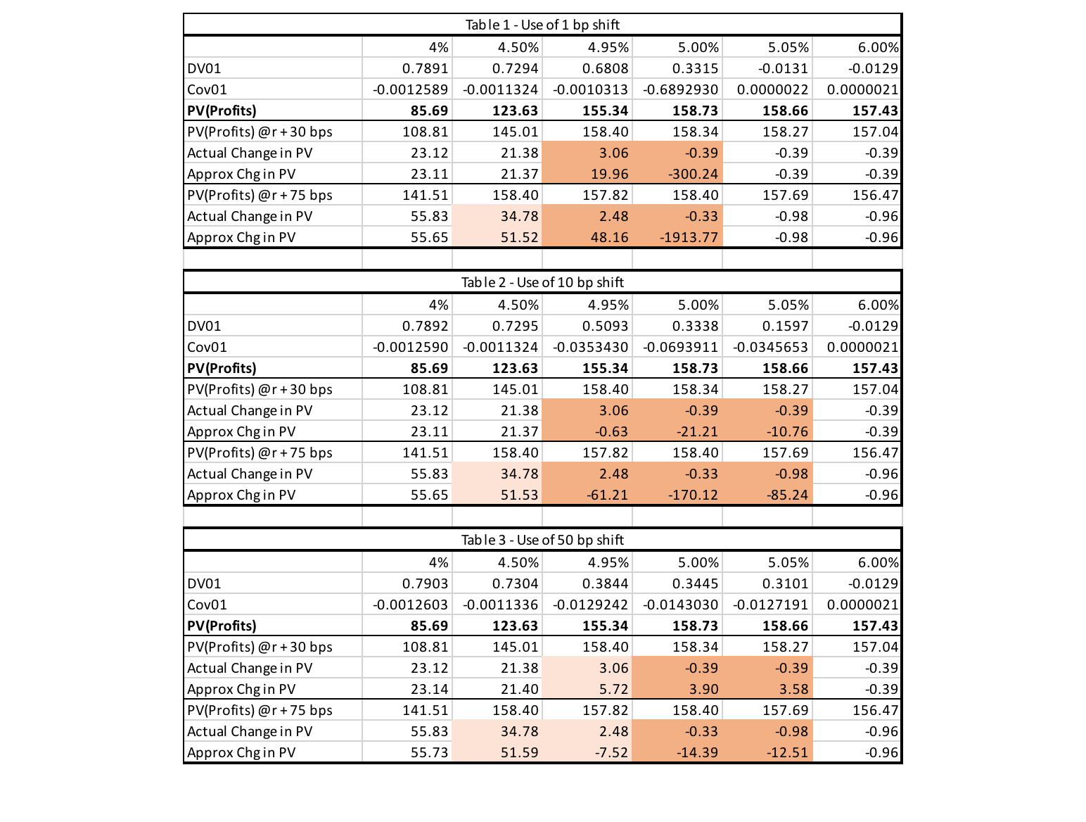
Now let us consider what happens if the shift size used in the calculation of DV01 and CV01 is larger. Table 2 provides the results for a 10-bp shift while Table 3 provides results with a 50-bp shift. For now, let’s consider a 50-bp shift (Table 3). Obviously, there is a higher chance that the rates used in the calculation of DV01 and CV01 will be on the opposite sides of the inflection point. This means that we are using a quadratic function that is neither close to the one that fits the values before the inflection point nor the one after. It is some combination of the two. Due to the fact that this function reflects a bit of both quadratic functions, it slightly improves on the approximation. For example, when the current rate is 4.95% the use of a rate increase of 30 bps produces a value change of 5.72 (compared with 19.96 using 1-bp shift) against the actual value of 3.06. And when the rate increase is 75 bps it produces a change of -7.52 (compared with +48.16 using 1-bp shift) when the actual change is +2.48. Note that while the error is reduced, the approximation is far from accurate and cannot be relied on for any decision making.
It should be noted that the above example was very simplistic to highlight the issue. With various assets and liabilities, one normally would not produce such graphs to identify to what extent one can rely on the metrics and at what rate shifts the inflection points may occur. Additionally, when matching duration and convexity of assets and liabilities one should realize that these metrics can be relied upon for different ranges for the assets vs. liabilities. Thus, the range that can be relied upon for surplus is the intersection of the validity range of assets and liabilities (smaller than either range). I further recommend evaluating these metrics directly for the surplus, if possible, as opposed to assets and liabilities separately. In the next part of this multipart article, I will provide a technique to identify where these inflection points occur and how one can adjust the metrics to estimate the value of the instrument for rate shifts that would cross the inflection point.
Statements of fact and opinions expressed herein are those of the individual authors and are not necessarily those of the Society of Actuaries, the newsletter editors, or the respective authors’ employers.
Dariush Akhtari, FSA, FCIA, MAAA, is chief actuary at Converge RE. He can be contacted at dakhtari@converge-re.com.