
Enhancing the Pedagogical Utility of Tables in Actuarial Teaching
By Russell Jay Hendel
Expanding Horizons, June 2021

Acknowledgment to the SOA for allowing reprinting portions of the corresponding presentation in ARC 2020. Statements of fact and opinions expressed herein are those of the individual authors and are not necessarily those of the Society of Actuaries, the editors or the respective authors’ employers.
Abstract
This article studies several pedagogical uses of tables, particularly as they apply to actuarial teaching. We start with a familiar use of tables, facilitation of comparison and contrast, and then journey to unexplored territory: the use of tables to facilitate remediation, to write good problems, to facilitate organization of complex problem solutions or professional papers, and to enable comprehensiveness and inspire intuition in complex multiparameter rules. This article will provide instructors at every level with something new and useful.
Introduction
Most instructors are familiar with tables as a vehicle of pedagogy. They know that it is good to use tables. But what exactly do tables accomplish?
Because tables are intrinsically two-dimensional, a table and narrative with the same information will not provide the reader with the same and quickest access to that information. The table provides faster access to many questions of comparison and contrast, something that bullet points and narrative cannot do.[1]
This article makes explicit, illustrates, and summarizes half a dozen uses of tables. It starts with the most familiar use. These initial examples precisely articulate the advantage of the table approach. As we proceed, we will look at lesser-known uses of tables.
Tables are important and frequently used. A recent survey in one journal of several hundred articles and several thousand pages going back 10 years showed that among papers that use tables, they are used 50 percent more frequently than graphs.[2]
Many books discuss the best way to present data visually in graphs, charts, or tables.[3] However, we will focus exclusively on tables. Furthermore, we are not primarily concerned with making a given table better looking by focusing on spacing, formatting, and display; rather, we are concerned about the very raison d’etre—the function—of the table in pedagogy. Therefore, the modest tour provided by this article will benefit both the experienced and novice instructor; moreover, knowledge of how to skillfully use tables benefits the professional writing of articles as well as pedagogy.
Throughout this article, examples are taken from the preliminary Society of Actuary examination tracks (including Calculus). It is assumed the reader is familiar with the courses, standard textbooks, notation and methods used.
Tables for Comparison and Contrast
We start with the most obvious advantage of tables: comparison and contrast. A straightforward illustration of this, from the Society of Actuaries (SOA) Financial Mathematics (FM) course, is presented in Table 1.
Table 1
Excerpt From a Table of Money Growth Methods in the FM Course

Note: In each cell, the top line represents time; the bottom line represents the accumulated amount in the account at time n, with A(n) the accumulation function.
A narrative approach to instruction would not automatically allow instant comparison and contrast between formulas. The table approach to instruction allows a student to see instantly that the formulas for compound interest and discount differ in signs in two places This is useful to facilitate avoiding student errors. Multiple similar examples are easy to produce.
Tables for Evaluation of Pedagogically Challenging Problems
Consider the following two problems from the Money Growth topic in FM.
I: What is the accumulated value of $1,000 invested for 2 years at an effective rate of 10%.
II: What is the accumulated value of $1,000 invested at time t = 3 for 2 years at an effective rate of 10%.
At first blush, the two problems appear identical in difficulty. However, the table concept shows that Problem II is superior.
The solution to Problem I is A(2) = 1,000 * (1.10)2. Furthermore, if Problem I were asked again using another money growth method—simple discount, constant force, etc.—the formula for computing the answer would only differ in the money growth function used: A(2) = 1,000 f(10%,2) where f(i,n) is the money growth accumulation function for the particular money growth method used at rate i (interest or discount) and for a duration of n years. We might summarize this by saying Problem I does not differentiate the accumulation functions of different money growth methods.
The situation is different for Problem II. To clarify this point, we consider two versions of Problem II using two different money growth methods.
IIA: What is the accumulated value of $1,000 invested at time t = 3 for 2 years at an effective rate of 10%, with the default accumulation function a1(i, t) = (1 + i)t.
IIB: What is the accumulated value of $1,000 invested at time t = 3 for 2 years using an accumulation function a2(t) = (1 + t)0.5.
Problems IIA and IIB have intrinsically different solutions. Problem IIA can be, and is usually, solved, using the relative time between the deposit and withdrawal, 2 years: A(5) = 1,000 a1(10%, 2). But Problem IIB cannot be solved this way. Problem IIB requires the use of absolute time. For this problem, A(5) / a2(5) = 1,000 / a2(3), implying A(5) = $1,224.75.
In terms of teaching the material, the correct pedagogical approach would be to add a column to the table of money growth functions commenting on the use of relative vs. absolute time. Such a column would also consider conventions of language. Table 2 presents an excerpt from the modified table.
As can be seen from this example, the table and the problem set synergistically interact. The table evaluates each problem as blasé or challenging. The challenging problems, in turn, inspire adding columns to the table, thus enriching the pedagogical experience.
Table 2
Excerpt From a Modified Table of Money Growth Methods in the FM Course
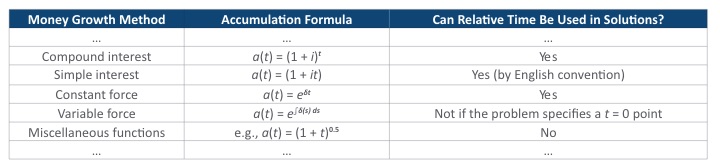
Note: The last column is multivalued (not just yes-no).
Tables as an Alexa, Assisting in Remediation
The clever and skillful use of header prompts can supplement, perhaps even replace, office-hour remediation. To develop this idea, we focus on a specific problem in the Long-Term Actuarial Mathematics (LTAM) syllabus.[4]
For a special 3-year temporary life annuity due on (x), you are given:
(i)
Table 3
Data Table for Question #114 in Exam MLC Sample Questions
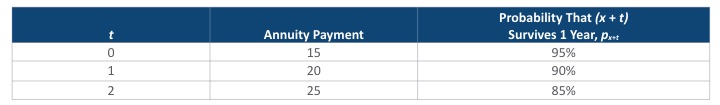
(ii) i = 0.06
Calculate the variance of the present value random variable for this annuity.
Instructors are familiar with the following, perhaps typical, office-hour dialogue:
Student: I am having trouble with this problem
Instructor: Do you need review on how to compute a variance? That is part of the course prerequisites.
Student: No, I remember how to do that. I just don’t know where to begin.
Instructor: Well, what is the distribution in this problem?
Student: Distribution? There is no distribution, just some probabilities of living 1 year.
Instructor: That is the key to solving your problem. To compute a variance, you need a distribution.
Student: But the problem did not give a distribution.
Instructor: Then you have to find it. Did the problem give a universe of events?
Student: No.
Instructor: I disagree. What event triggers payment in this problem?
Student: Death of the insured.
Instructor: When can the insured die?
Student: Between 0–1, 1–2, past 2.
Instructor: Aren’t those mutually exclusive exhaustive events?
Student: Yes?!
Instructor: Then calculate the probabilities of these events, ensure their sum is 1 and you will then be able to compute the variance.
Student: I should have thought of that before coming.
An instructor having gone through this discussion in various forms several dozen times can encapsulate it in skillfully created table headers and provide these as instructional aids. The solution to this problem is presented in Tables 4a–4c, with the headers mirroring questions taken from the instructor-student dialogue just presented.
Table 4a
Main Solution Table to Question #114
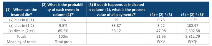
i The values of columns (2) and (3) come from Tables 4b and 4c.
ii Var(X) = E(X2) – E(X)2 = 114.2.
Table 4b
Calculation of Probabilities of Events of Death
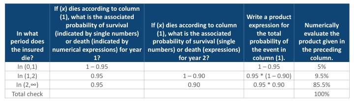
Note: The last column in this table feeds into column (2) of Table 4a.
Table 4c
Calculation of Possible Annuity Payouts
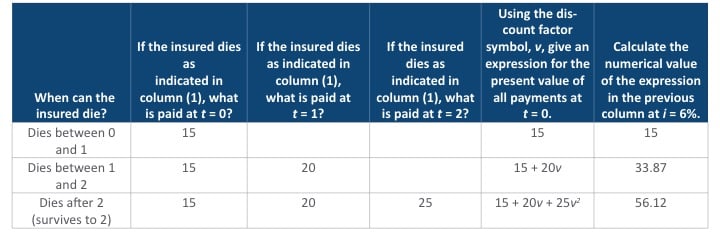
Note: The last column of this table feeds into column (3) of Table 4a.
The use of tables to assist in remediation is varied; this example shows one approach. By presenting the material like this, one encourages students to think in a certain way, thereby avoiding the confusion that leads them to seek extra help. Instructors can typically tailor solutions to what they need based on course complexity and student abilities.
Tables as Highway Stops on a Long Narrative Road
In the previous section we solved a problem using three tables; contrastively, the SOA uses one table in its solution. This points to an important use of tables. They provide organizational highlights, or resting places, in a long narrative. This applies to complex problems taught in class; it also applies to narrative in written papers.
The section title provides an analogy with a highway. Yes, the stops on the highway support numerous functions, such as food, gasoline and restrooms, but a main advantage is that they break up a long road and afford people the ability to just breathe and stretch their legs.
This contrasts with the traditional approach of using tables: first, write the narrative, and then throw in some graphics and tables to please readers.[5] Here, we advocate the opposite: if you have a complex problem to solve, first create a series of tables that solve it. This series of tables becomes a skeleton around which to write the narrative, to fill the skeleton with flesh, to make the story soft and bouncy.
The undergraduate curriculum is strewn with such highway problems. Some common examples are the test for statistical significance and the complete graphing of a third- or fourth-degree polynomial. The current instructional approach—to give partial problems such as “sketch the region that is concave downward and increasing”—is pedagogically harmful and not correct. Throw the students in the water; let them swim, not just get their feet wet; let them navigate the entire path of the problem. However, to expect this from students, one must prepare them for these complex problems by emphasizing the role of the table as a navigational tool.
We will close this section with some reflections about the role of the actuarial instructor. Consider two students in your classes: one is interested in being a banker, and one is interested in being an actuary. If your goal is to prepare a student for, say, a banking job, it suffices for them to know how to plug into formulas or create a spreadsheet. Most banking work being done is known in advance, and therefore you can simply teach the tools needed every day.
Using the language of the educational hierarchies, the banker must be adroit in the retrieval, comprehension, and application of known financial material.[6] However, the actuarial student must be able to utilize, analyze, and synthesize knowledge. The successful actuary does not know all of their daily work in advance. Hence, the actuary must be taught component skills, have the ability to analyze each new problem into components and synthesize a new solution that solves that problem. Therefore, the approaches to teaching future bankers and future actuaries are different.
Thus, actuarial teaching should continuously reflect a goal of analysis and synthesis. The solution to the problem presented with Table 3 is a model. The student would realize that to solve the variance of a random variable they need an event space, a distribution and values of that random variable (Table 4a). Such an analysis immediately gives rise to two needs: a table for the distribution (Table 4b) and a table for the present value random variable (Table 4c). It is precisely by presenting the solution as a sequence of three tables that we encourage the analysis and synthesis the student will need. It is most noteworthy that the solution to this problem on the SOA website misses this golden opportunity; only one solution table is presented with three footnotes of computations added. This, as just remarked, is inconsistent with actuarial pedagogical goals.
Tables Facilitating Intuition and Comprehensiveness
To introduce the main idea of this section, consider the topic of identifying minima in Calculus. The following dialogue presents some typical errors poorer students might make and how instructors might respond.
Student #1: But f′= 0 at X = x0. So x0 is a minima.
Instructor: f′ = 0 is not sufficient. You have to check the values of f″.
Student #2: The function is linear— f′ > 0 everywhere—so there is no minima.
Instructor: You still have to check the boundary points.
Student #3: But f″ = 0 is an inflection point and hence not a minima.
Instructor: Inflection points may sometimes be extrema.
These hypothetical dialogues point to general issues with a multiparameter rule—in this case, the multiparameter rule for minima. The dialogue identifies the following deficiencies in the way calculus is sometimes taught.
First, many calculus texts may overemphasize the role of f′ = 0 coupled with f″ > 0 as determining minima. These texts may have many examples illustrating this rule and many exercises allowing students to practice their derivative skills. Second, the other tests for the minima—testing boundary points and testing inflection points—may only receive cursory mention, and there may be insufficient exercises for these other cases. Third, not all textbooks present the overall rule comprehensively; some textbooks may leave checking boundary points and other parts of the complete rule to exercises and not include them in the textual narrative. All this leads to confusion for students, who are not certain for what they are responsible.
These criticisms apply to any multiparameter rule. Tables can assist instruction and student mastery in two ways. Table 5 presents an example table, a table of examples. Such tables, or their equivalent, are useful, especially in the constructivist approach to teaching.[7] Constructivism posits that students can’t be taught mathematics; the instructor can at most provide students with examples so they can construct the theory themselves. Constructivism, using the method of guided discovery, presents students with sufficient examples for them to construct in their own minds the necessary concepts needed to address certain problems.[8]
Table 5
Various Examples of Functions, Their Attributes, and Their Minima Status at X = 0
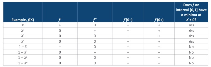
Note: Derivatives in columns 2 and 3 are evaluated at 0. The notation f′(0–) refers to the function f′ evaluated a little bit to the left of 0.
Using these examples, we can abstract a comprehensive principle, expressed as a Boolean rule, that applies to our problem hypotheses: functions are continuously differentiable on the entire real line, but minima are taken over an interval, [0,1]. There are algorithmic methods to extract from a complex example table a Boolean rule that is simultaneously comprehensive and intuitive. These methods are presented in many standard undergraduate texts.[9]
A complete table based on Boolean attributes corresponding to a traditional disjunctive normal form is too complex to provide useful information. What is needed instead is the prime implicant normal form (PINF), a technical term defined in textbooks.[10] Two popular methods for extracting the PINF from a complete truth table are the Quine-McCluskey reduction rules and Karnaugh maps.[11] The resulting Boolean rule for determining minima on the interval [0,1] of a function continuously differentiable on the real line, that rule expressible as a Boolean function, is presented in Figure 1.
Figure 1
Complete Test for Minima of a Continuously Differentiable Function on Interval [0,1]

Note: In this figure, juxtaposition refers to conjunction; + and – by themselves refer to the sign of values of the function (i.e., positive or negative). Function evaluation is at the point mentioned in that part of the rule—P, 0 or 1. P is an arbitrary point inside (0,1). P+ and P– refer to a point near P. For example, the last disjunct says, “We are at a right boundary point (which is 1), and f′ to the left of that point is negative.”
The following conclusory points should be noted on multiparameter rules:
- Local Boolean rule: Some approaches avoid a Boolean rule and instead use a global approach (e.g., evaluate f at all critical points—including f = 0, f″ = 0 and boundary points—and ascertain the minima). However, the rule in Figure 1 is local.
- Comprehensiveness: The rule completely describes all things to be checked for finding the minima over a finite interval of a continuous function with a continuous derivative on the entire real line. Notice that the last two disjuncts, boundary tests, are not found explicitly in all textbooks but are nevertheless useful. A key point for an instructor is that each prime implicant in the aforementioned function should be addressed in the course in both narrative and exercises.
- Intuitiveness: The example table doesn’t succinctly identify core drivers of being a minima. The prime implicants in the rule presented in Figure 1 provide needed intuition. For example, the familiar assertion that a minima occurs if f′ = 0 and f″ > 0 is the first prime implicant in the rule (after expansion) but with the important condition “non-boundary point” omitted. Further intuition is provided by the second prime implicant, which states that at a non-boundary point P, f′(P) = 0, and for a little bit to the left and right of this point, the first derivative is negative and positive, respectively. This could prove useful if the second derivative has discontinuities or is not defined. Similar remarks can be made on the last two prime implicants. It is noteworthy that the content of these prime implicants is not always mentioned in texts, thus pointing to a pedagogical problem which can be remedied by tables.
Conclusion
Tables can be used to compare and contrast, identify superior problems, improve or supplement remediation, improve the organizational clarity of a long narrative or solution, and provide comprehensiveness and intuition. Every instructor, independent of their level, will find something useful here.
Russell Jay Hendel, PhD, ASA, is adjunct faculty III at Towson University, where he assists with the Actuarial Science and Research Methods program. He can be reached at RHendel@towson.edu.