
Exploiting While Exploring: An Introduction to Bayesian Optimization
By Nick Hanewinckel
Predictive Analytics and Futurism Section Newsletter, June 2021

Most actuaries, data scientists, and unicorns (i.e., both) got their start with parametric statistical models. The classic example is the ordinary least squares (OLS) method to fit linear regressions. These generally have closed-form solutions across all modelling problems.
Later, we begin to move up the machine learning spectrum and encounter our first hyperparameters. Perhaps we first learn of L1 (LASSO) and L2 (Ridge) penalty hyperparameters. Perhaps next we learn of elastic nets that combine these penalty hyperparameters with α (penalty weights). We may even move further to complex gradient boosted machines (xgboost) with even more parameters.
This presents us with a tricky problem: these model fits may be expensive (time/compute resource-intensive) and the hyperparameter space is huge! How can we find the optimal fit?
Definitions and Side Notes
If this is new to you, let’s define what a hyperparameter is versus a more familiar model parameter. For a linear regression, the parameters are the βs (coefficients) that we solve in order to estimate. The data and model form fully specify these coefficients (remember: OLS is just a solution to a calculus minimization problem). A hyperparameter is a parameter of the machine learning process itself independent of any data. No matter how smart you are, you simply can’t figure out mathematically what values will lead to the best fit. So as always, the proof is in the holdout set.
Also important: As these models are complex and nonlinear, there will not be a unique set of parameter values. Perhaps a model can learn just as well using 500 trees and a slow learning rate as it can from 100 trees and a faster learning rate.
Finally, some areas of the parameter space may be known to work well for given problems/types of data. This is another way to say that some level of expertise and collaboration is helpful. Nevertheless, the aim of this article is to show how you might narrow down your parameter space with little prior knowledge.
Other Methods
Before we get into Bayesian methods, there are other methods to consider. A traditional grid search simply fits candidate models for all values in the given parameter space. However, as the number of parameters increases, the number of trials needed to test the whole space becomes combinatoric. This is made worse by the expensive nature of fitting. This is often called the curse of dimensionality.
Another approach is a random grid search where a sample of parameter values are naively drawn from the search space. The problem with this unsupervised method is that each trial is independent—not at all improved by the information from prior fits.
Finally, some models have solvable gradients, so gradient descent can be used to estimate the next “sweet spot.” Unfortunately, only specific models (e.g., neural nets) can use this method. The method assumes concavity of the gradient, which is not accurate for many powerful model families. Fortunately, the Bayesian technique is model-agnostic.
Bayesian Optimization
The basic idea is to analyze the results of a set of trial models and choose the next set of hyperparameters where fit is likely to improve. Since we do now know the gradient of the parameter space, we use a surrogate model to model our model’s hyperparameters. Specifically, we choose a Gaussian process as our prior distribution. This prior along with a likelihood function for prior observations creates a posterior distribution that we can use to predict new values for the parameters where we expect the model to fit well.
So how do we define the ideal next point? In one basic approach, called active learning, we always seek to reduce uncertainty. To do this, we choose the point with the highest variance (often far from the original point).
The issue with active learning is that we are maximizing our exploration of the parameter space, which may be computationally expensive. Basing our process on the uncertainty (not quality) of predictions means we essentially are doing a stepwise search of our modelling space without exploiting the good fits we find along the way.
To balance exploration versus exploitation of the parameter space, the Bayesian approach uses acquisition functions as the metric to evaluate next steps. These functions themselves have a parameter. We hope to explore smart ways to choose these parameters to avoid a long process of hyperparameter tuning.
Acquisition Functions
We will skip the gory statistical details, but the acquisition functions are often intuitive. They include: expected improvement, probability of improvement, upper confidence bound, lower confidence bound, and others. I will give an example of EI, PI, and LCB. EI and PI use ξ and LCB uses κ. Higher values for these parameters lead to more exploration (sampling across the space favoring variance) and lower values lead to more exploitation (more likely to search the space near prior optimal results).
Example—Mortality Model
For our example, we will use an xgboost model along with Python’s scikit-optimize package with ILEC mortality data taken from http://cdn-files.soa.org/research/2009-15_Data_20180601.zip. This will be a Poisson (death count) model scored with negative log-likelihood. To make the data and problem more manageable, we take a subset of this data and restrict it to issue ages [40,60) and duration < 10. Python was chosen as scikit-optimize has a strong BayesSearchCV that integrates well with xgboost and scikit-learn models as well as other functions such as partial dependence plots.
When I worked in R, I often wished for a Bayesian grid search library. Since then, I have become aware of the rBayesianOptimization package, though this hasn’t been updated in several years. The tune package is less than a year old and is part of the tidyverse family of packages. I have not used either, but numerous examples exist online that you can compare with the code for this article.
To follow along, the full code from this exercise is hosted at https://github.com/hanewinckel/OptimalGridsearch.
It’s less important how the model actually fits overall for this article. This example is not necessarily the best model type, feature set, or parameter space for the given problem. We want to analyze the optimization process itself. In general, if optimization output references the “test set,” it is referring to the average scores for the cross validation’s holdout set across all folds.
Model Parameters
An xgboost model has a large number of parameters; it is a great example of a model where the size of the parameter space poses a problem. To focus on our search, we will only alter four (sampled from a uniform distribution unless noted otherwise):
‘model__n_estimators': Integer(10,1000),
'model__gamma': (1e-8, 1e+3, 'log-uniform'),
'model__max_depth': Integer(2, 8),
'model__learning_rate': Real(0.005,0.5)
There are many other parameters (including L1/L2 penalties and sampling behavior) and I invite you to clone the git repo in the link above and experiment with even bigger grid searches.
Global Grid Search
In a perfect world, we could somehow know the optimal parameters to compare with our work. Since this is not possible, I fit a “global” Bayesian grid search with 50 iterations. This will at least give an idea of the optimal parameters and score. By default, a random draw of acquisition functions will be used to pick the next point. We will then compare this with grid searches done for specific acquisition functions and parameters.
As this was a simple model, the best fit was found in the 12th iteration at a score of -0.00619. Specific experiments use 10 iterations per acquisition function, which would not be enough in this case.
We can see a plot of the scores by iteration (Figure 1):
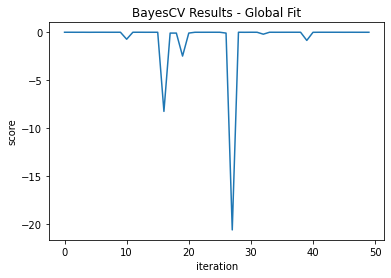
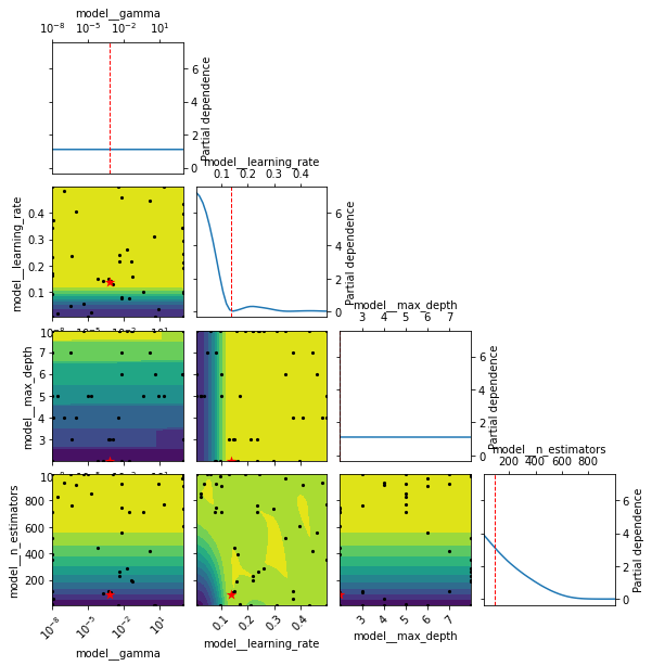
This doesn’t directly tell us if we are exploring or exploiting, but we do know that the model continues for 38 iterations after the ideal point. We can also produce a partial dependence plot for the estimated objective function—the red star is the optimal point so you can see what parameters led to this (Figure 2):
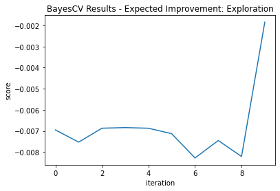
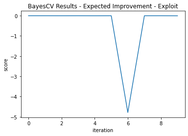
Acquisition Function—Expected Improvement
Two grid searches of 10 iterations each are performed with ξ = 0.3 to focus more on “exploration” and ξ = 0.01 to focus on “exploitation.”
Our exploration version didn’t find the optimal point until its final iteration. However, this model score was -.00185, significantly better than the global fit.
The exploitation version got lucky and found its optimal point on its first iteration. It was not so lucky in that it didn’t explore more and its best score was - 0.00682, not quite as good as the global search.
This shows why exploration can be valuable—particularly in unfamiliar space. Note the differences in fit trajectories when exploring versus Exploiting (Figure 3 and Figure 4):
Acquisition Function—Probability of Improvement
Two grid searches of 10 iterations each are performed with ξ = 0.5 to focus more on exploration and ξ = 0.05 to focus on exploitation.
Both methods had very similar measures: -0.00683 for exploring, -.00685 for exploiting. The by-iteration plots don’t tell us much, but looking at the fit log we see much greater variation in the parameters tried under the exploration-centric parameter.
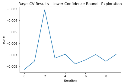
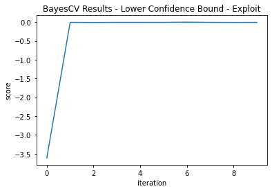
Acquisition Function—Lower Confidence Bound
Two grid searches of 10 iterations each are performed with κ = 2.3263 to focus more on exploration and κ = 1.38 to focus on exploitation. These correspond to normal Z scores.
Here, the exploitation method found better fit (-0.00126 vs -0.00309; the best score yet).
You can see here that the exploratory parameter gets us very close in iteration two, but does not exploit it; rather, it jumps around the parameter space. The exploiting parameter finds a good fit by duration two, but it locks on to this area of the modeling space and finds an even better one (Figure 5 and Figure 6):
Conclusions
Two important things appear contradictory: 1) In some sense you “can’t go wrong” with a Bayesian search. Slightly different parameters still lead to good model scores; 2) At the same time you can’t just “point” a Bayesian grid search at your problem and expect it to work like magic.
Some ways to deal with this include simply running more iterations with a wider parameter grid. This is computationally expensive, but perhaps you could let a set of models run overnight and get what you’re after. At the same time, if you are digging in the wrong field, you’ll never hit gold.
To fix this, we can also employ a mix of exploration and exploitation. For our first grid searches, we can take an exploratory approach. Then, when we know what parts of our parameter space produce good results, we can focus more on exploitation.
Perhaps another way to deal with this is to try using a bit of actuarial judgment. As with many actuarial problems, it’s best to combine your knowledge with those of others. Perhaps see what parameters worked for other data scientists solving similar problems. And while we can’t formulaically solve for our parameters, we can use some guidelines. If you have a more complex problem with more data, you may need to increase your maximum depth or number of trees. And when you do that, you risk overfit, so you may have to increase penalties. If you have a lot of predictors, you may need to explore sampling parameters.
I invite you to pull this repository and play around. If you create something you think is interesting, go ahead and open a pull request!
Thanks for reading!
Statements of fact and opinions expressed herein are those of the individual authors and are not necessarily those of the Society of Actuaries, the editors, or the respective authors’ employers.
Nick Hanewinckel, FSA, CERA, MAAA, is AVP and lead data scientist with SCOR Global Life Americas. He has worked in predictive analytics for life insurance for several years and is a council member of the PAF Section, treasurer, and newsletter editor. He can be contacted at nhanewinckel@scor.com.